Lerner2022

This is a submitted version of the manuscript. The final publication is available at www.degruyter.com

https://doi.org/10.1515/jqas-2022-0043

A Peculiar Phenomenon and its Potential Explanation in the ATP Tennis Tour

Finals for Singles

Abstract

The ATP finals is the concluding tournament of the tennis season since its initiation over 50

years ago. It features the 8 best players of that year and is often considered to be the most

prestigious event in the sport other than the 4 grand slams. Unlike any other professional tennis

tournament, it includes a round-robin stage where all players in a group compete against each

other, making it a unique testbed for examining performance under forgiving conditions, where

losing does not immediately result in elimination. Analysis of the distribution of final group

standings in the ATP Finals for singles from 1972-2021 reveals a surprising pattern, where one

of the possible and seemingly likely outcomes almost never materializes. The present study uses

a model-free, optimization approach to account for this distinctive phenomenon by calculating

what match winning probabilities between players in a group can lead to the observed

distribution. Results show that the only way to explain the empirical findings is through a

“paradoxical” balance of power where the best player in a group shows a vulnerability against

the weakest player. We discuss the possible mechanisms underlying this result and their

implications for match prediction, bettors, and tournament organization.

Keywords: betting, model-free approach, round-robin, tennis

1. Introduction

The use of data analytics in professional tennis has become increasingly more common over the

last decade. More and more players are taking advantage of advanced statistical analyses to

improve their game, whereas media outlets, helped by software giants (e.g. I.B.M) use the data to

present the audience with enriched analysis of matches in real time (Larson and Smith 2018).

These analyses, however, have been mostly limited to the development of models and metrics to

describe broad aspects of the game, such as predicting the outcomes of tennis matches (e.g.,

Ingram 2019; Klaassen and Magnus 2003; McHale and Morton 2011; Spanias and Knottenbelt

2013; see review by Kovalchik 2016), revising ranking systems (e.g., Bozóki, Csató, and Temesi

2016). ; Irons, Buckley, and Paulden 2014), or settling popular disputes with interest to pundits

and general audiences (e.g., Radicchi 2012). While a few studies have examined more specific

aspects, such as success rates of elite players in elite tournaments (e.g. Gallagher, Frisoli, and

Luby 2021; Leitner, Zeileis, and Hornik 2009; Wei, Lucey, Morgan, and Sridharan 2013), their

approach remained top-down: developing a model and then applying it to a particular dataset

chosen for its prominent status and visibility.

Much less common are bottom-up approaches, which begin with identifying local, unique

statistical patterns in the field, and then examine whether they could be accounted for by

mechanisms that have broader implications on the sport. The current work attempts to illuminate

such a unique pattern appearing in the ATP Finals tennis tournament for singles, explain its

possible sources through a “model-free” statistical approach, and draw conclusions with possible

interest to players, ATP officials, tennis pundits and betting agencies. To the best of our

knowledge, this is also the first academic attempt devoted specifically to identifying and

explaining statistical patterns in the ATP Finals in tennis.

The ATP finals (please see https://www.nittoatpfinals.com/en/heritage/history) is the

concluding tournament of men’s tennis calendarial year, organized by the Association of

Professional Tennis (ATP). It has been taking place regularly since 1970, usually during

November (and, at some years in its first decade, during January of the following year), and

features the 8 players with the highest seeds in the ATP ranking based on performance during the

season. Given that only the players with the best results of that year are allowed to participate, it

is often considered to be the most prestigious tennis tournament other than the four Grand slams.

The ATP Finals are distinct from all other ATP-tour tennis tournaments in that they are

not entirely designed as a knockout system where every match ends up in the elimination of the

losing player. Instead, it employs a round-robin stage where the 8 players are organized into two

4-player groups, with each player playing against all other three in his group. Groupings are

based on the players’ seeding in an attempt to keep each group at a roughly similar level. As

such, the number 1 and 2 seeds will find themselves in opposite groups, as will the number 3 and

4 seeds, 5 and 6, etc. The two players ending up on top of each group by the end of the round-

robin stage then proceed to a regular knockout stage with semifinals (in which each group’s

winner faces the runner-up of the other group), followed by a final. Thus, during the group stage,

a player may lose a match – or even two – and still remain in the tournament. The two winners of

each group are determined by ordering their performance based on the number of wins, and, in

case of a tie, based on a cascade of additional measures, including number of games played

(mostly relevant in cases when a player skips an entire match due to injury and needs to be

substituted), sets won, head-to-head results and so on (see https://www.nittoatpfinals.com

/en/event/rules-and-format). Over the years, there have been several variations from this setup,

particularly during the first decade and a half of the tournament’s life. For example, in 1970-

1971 the tournament only had a group stage with one single group and no knockout stage

whereas during 1982-1985 it was conducted as a regular knockout tournament from start to

finish (https://www.nittoatpfinals.com/en/heritage/results-1970-1999); the finals have sometimes

been played as best-of-five sets rather than best-of-three like the rest of the tournament

(https://www.nittoatpfinals.com/en/heritage/results-2000-2021) ; the allocation of players to

groups based on seedings was not followed in the first few years; and the specific cascade of

tiebreak rules determining the ranking of each group in case players end up with the same

number of wins has seen some minor variations; but overall, the format has been quite stable for

over half a century of the tournament’s existence.

Our main concern in the current study is the peculiar statistical distribution of the final

standings of the group stage in the ATP Finals in singles, particularly as they relate to the

number of wins/losses. Since all 4 players play against each other for a total of 6 matches and

there is always one winner and one loser in a tennis match, the final standings can result in only

one of four outcomes

(i) One player winning all of his matches, one player winning two matches, one player winning

one match and one player winning none (3-2-1-0).

(ii) Two players winning two matches and two players winning one match (2-2-1-1).

(iii) Three players winning two matches and one player winning none (2-2-2-0).

(iv) One player winning three matches whereas the other 3 winning one match each (3-1-1-1).

The frequency of each of these outcomes could enlighten us about the balance of power

between players in an ATP Finals group. For example, if we assume the (highly unlikely)

scenario where all players are equally strong with each having a probability of exactly 0.5 to win

Here, we disregard the (somewhat uncommon) situation where a player gets injured and is substituted by another

player mid tournament, and treat it as if the same player was playing throughout. This is discussed later on.

a match, it can be shown that the expected frequency distribution of the final standings over the 4

possible outcomes will be [0.375 0.375 0.125 0.125]. In other words, it would be as likely to find

a 3-2-1-0 and a 2-2-1-1 standings, with each occurring 3/8 of the time, and it would be as likely

to find a 2-2-2-0 and a 3-1-1-1 standings, with each occurring 1/8 of the time.

Naively, one would assume that each of the possible outcomes would be at least

somewhat likely; however, when examining the standings over all groups across the years of the

ATP Finals’ existence, we find a highly skewed distribution, with the fourth outcome (3-1-1-1)

occurring in only 2 out of 92 cases, a frequency of merely 0.0217 (for comparison, in the ATP

Finals for doubles, played in a similar format, no outcome occurs less than 0.085 of the time; and

in the WTA Finals, the equivalent tournament in women’s tennis, all outcomes have frequencies

above 0.105);. Having such a low probability for a seemingly reasonable scenario (especially

given that the other scenario where one player wins 3 matches, 3-2-1-0, is very likely) deserves

explanation, as it may defy expectations set not only before the beginning of proceedings but

also while the tournament is already underway (with potential repercussions to betting patterns).

The following study attempts to explain this finding by examining what balance of power among

the players in a group, as expressed by their probabilities of winning a match against each other,

could result in such a peculiar group standing distribution.

2. Methods

Data on all match results in the ATP finals for singles were extracted from the official ATP

website (https://www.atptour.com/en/scores/results-archive). Relevant data included 46 out of

the 53 years of the tournament’s existence (1972-1981 and 1986-2021), when it was played with

a round robin stage that included two 4-player groups. In addition, when we needed to determine

the exact order of matches played, information was extracted from the sports statistics website

Flashscore (https://www.flashscore.com/).

We begin the analysis by computing the frequency of each of the 4 possible outcomes of

the group standings. Each tournament contributes two samples for the calculation (corresponding

to the two groups in each year), resulting in 92 samples over 46 years. The resulting distribution

was:

= [0.6739 0.2065 0.0978 0.0217] (1)

for the 3-2-1-0, 2-2-1-1, 2-2-2-0 and 3-1-1-1 outcomes, respectively.

is thus considered as the

empirical target distribution that we aim to explain in this study.

Next, we characterize the results of a round-robin group by

a vector with 6 values

…p

) representing the probabilities of a win by one player over another, which can be

displayed in the following matrix form:

Losing player

Winning player

1-p

We search for a value of

# that yields the target distribution of the group standings

outcomes. For simplification, we assume that the results of each of the 6 matches taking place in

an ATP Finals group in any year are independent of each other (i.e., each match depends on the

relative contemporary strength of the players involved, but not on the results of the other matches

in the group or any other results). While this is not necessarily the case, it is a reasonable

approximation for which some support is given later on. Again for simplicity, we ignore

instances where substitute players were used due to one or more players getting injured and

forced to quit the tournament, and treat them like any other sample. Substitutions are an

uncommon though not negligible phenomenon, occurring in 12 out of the 92 cases; however,

they do not change the basic win-loss statistics we target in this study and our conclusions are

valid even when discarding them from the calculations, therefore we report the results with all

data included. Finally, note that our approach intentionally ignores seedings since our goal is to

describe the patterns over all groups in the tournament’s history with no prior assumptions about

likely results based on previous performance in a given year. Seedings are addressed only at one

point when trying to estimate the stability of the statistics (see Results).

To estimate

#, we search for values of p

…p

that yield a distribution of group standings

%&$

that is as close as possible to the target distribution. We define the distance between the two

distributions based on the Kullback-Leibler divergence (D

; Kullback and Leibler 1951), which

gets a value of 0 when the two distributions are identical, or a positive value when they are not.

This turned the calculation into an optimization problem, where our goal is to find

(

that

minimizes the objective function D

)*+,-.

⃗

1 %

2 (2)

Similar results are achieved when using other objective functions to define the difference between the two

distributions, such as sum squared difference, City block distance (the sum of absolute differences in each

dimension), or the counterpart definition for Kullback-Leibler divergence,

𝐷

𝜃

(

𝑝

⃗

)

∥ 𝑇

⃗

+. D

was preferred

because it more naturally captures similarities between distributions and thus requires fewer repetitions to

effectively cover the parameter space.

A small additional correction is applied to the objective function due to the inherent

limitations on precision when using a finite amount of available data. Specifically, substantially

different values of

(

can bring the objective function close to 0 with only tiny disparities that do

not meaningfully reflect a higher likelihood of one set of

(

values over the other. To overcome

this, we set a threshold for the difference between

%&$

and

, below which the objective

function was manually set to 0. The difference was computed as the City block distance (see

footnote 2) between the two distributions, and the threshold was determined to be 1/92, the

resolution of the target distribution (given 92 data points, a City block distance between

(

and the target distribution that is higher than 1/92 suggests that

(

is, in fact, closer to

another target distribution that could have been produced with the same amount of data).

Estimation of

# was performed numerically using the Nelder-Mead simplex algorithm.

The optimization algorithm was run on Matlab 2021a (Mathworks) using the built-in fminsearch

command. Since the algorithm’s output is sensitive to initial conditions, we repeated the

optimization procedure 50,000 time, each time starting with a random initial condition

, to

assure a good coverage of the whole parameter space (additional runs did not change the results

much further, nor did dividing the parameter space into an evenly spaced grid and setting the

initial conditions to each of the grid edges). Other analyses described in Results, including

Principal Component Analysis (PCA; Abdi and Williams 2010) and K-means clustering (Lloyd

1982) were carried out using the Matlab commands pca, kmeans and kmeans_opt.

3. Results

We first tested our assumption that the group standings in tournaments are approximately

independent of each other. To that end, we computed the joint probability distribution of the two

group standings of each year (across the 46 years of available data), which includes 10 possible

outcomes (all pair combinations of the 4 possible final standings, disregarding order; for

example, one outcome is when the two groups in a single year both end with 3-2-1-0 standings;

another is when one group ends with 3-2-1-0 and the other with 2-2-1-1; and so on). We then

computed the expected frequency of the joint distribution had the two groups been equally and

independently distributed, using the target probability T extracted from the full dataset. These

two joint distributions are presented in Figure 1, ordered by the magnitude of the expected

frequency of each outcome.

As can be seen, with minor exceptions, the two distributions resemble each other

considerably. This was confirmed using a chi-square goodness of fit test comparing the two

distributions (multiplied by 46, the number of data points), yielding a non-significant value

(

(3, N = 46) = 0.881, p = 0.83)

. While this test is not a strong guarantee that the groups are

indeed independent (given the limited data), it serves as a sanity check to confirm that this

approximation is not completely unrealistic.

---- Place Figure 1 Here ----

We further evaluated the assumption of equality and independence of the final group

standings each year by distinguishing the groups based on players’ seeding. While there is no a-

priori “correct” way to differentiate between the two groups of each year’s tournament as if

Given that many of the possible outcomes yield an expected count that is smaller than 5, the minimum value

required for reliably applying a chi-square test, we pooled together the 7 least-frequent outcomes into one big

category, yielding a total of 4 outcome categories used in the statistical test. We also verified this result by running

Fisher’s Exact test on the full 10 categories (since this test requires integers representing exact number of

occurrences, the values of the expected frequency were rounded). The result showed, again, that the two

distributions were not significantly different (p = 0.97).

representing samples of two different variables, differentiating by seeding presents a natural and

appealing option since in the majority of years, there has been a deliberate attempt to maintain a

roughly equal draw by making the groups as equal as possible in respect to their seedings (as

mentioned earlier in Introduction). We therefore differentiated between the groups that included

the number 1 seed (“Group 1”) and the groups that included the number 2 seed (“Group 2”) and

separately analyzed their performance over the years. Only 39 of the 46 years of available data

were included in this analysis since for 7 years groups were not equaled based on seedings. We

examined three measures of performance for each group: (1) group standings distribution over

the years; (2) probability of the players in the group reaching the finals; and (3) probability of the

group yielding the eventual winner of the tournament.

We found that the distribution of group standings for Group 1 was [0.6667 0.1795 0.1026

0.0512] whereas for Group 2 it was [0.6410 0.2308 0.1282 0]. Fisher’s exact test showed there

was no significant difference between the two (p = 0.62), nor was there a difference between

each of them and the target distribution

calculated over the entire data (both p’s> 0.85). The

probability of a player from one of the groups reaching the final was 0.526 for Group 1 and

0.474 for Group 2, and the probability of a player from one group winning the tournament was

0.538 and 0.462 for Group 1 and 2, respectively. Fisher’s exact test showed, again, that neither

difference was significant (both p’s>0.78). In summary, when differentiating the groups based on

seedings and separately evaluating each group’s performance over the years, we found that they

exhibit roughly the same performance overall, with similar distributions of final group standings

and success in yielding the finalists and winner of the tournament.

Having verified that the preliminary assumptions of our approach are acceptable, we next

moved to perform the main analysis of fitting a value for

#, the vector of win probabilities of

each match in a group, using the numerical optimization procedure described in Methods. The

calculation produced a variety of solutions for

# reflecting a range of values that perfectly

minimized the objective function (up to the possible precision point; see Methods). The range for

each p

…p

values across the 10,297 perfect solutions found is displayed in a color chart in

Figure 2, corresponding to the winning-losing player matrix presented in Methods. Rows were

ordered from the best player in the group (top) to the weakest player (bottom), and the range of

values for each p

is displayed within the corresponding cell sorted from the highest (center) to

lowest (edges).

---- Place Figure 2 Here ----

As is evident in Figure 2, across the range of possible values, the strongest player in the

group was always highly likely to win against the 2

- and 3

-best players (with probabilities

that are predominantly between 0.85-1), while the 2

-best players almost always won against the

weakest player in the group (with a probability that is close to 1). The matches between the 2

and 3

-best players, as well as the match between the 3

-best and the weakest player, were more

varied with probabilities that predominantly ranged between 0.6 and 1. With one notable

exception, the probabilities for a win generally tended to have the expected pattern of becoming

higher and higher for each player as they faced the weaker players of the group, evident by an

overall increase in values in each row from left to right. The one notable exception was the

match between the strongest and weakest players in the group (upper right and bottom left cells):

For every possible solution, this match never favored the best player decisively, with

probabilities that barely reached 0.8 and were most often closer to 0.75 or lower. In other words,

the optimization analysis led to a range of results with one peculiar core theme: a relative

weakness of the best player in the group when facing the weakest player. One additional peculiar

result was the absolutely dominance of the 2

-best player over the weakest player. While an

advantage is expected, this was the most one-sided matchup in the whole matrix (higher, for

example, than any of the winning probabilities of the best player), and it remained uniformly

high for all possible solutions.

---- Place Figure 3 Here ----

To gain deeper understanding of the core structure of the results, we performed PCA over

the various solutions for

#. We found that the majority of the variance in the solutions lied in the

first principal component, indicated by the first eigenvalue being more than 5 times larger than

the 2

eigenvalue, and more than an order of a magnitude larger than the rest of the eigenvalues

(Figure 3A). This first principal component almost exclusively modulated the probabilities of the

-best player’s matches. As seen in Figure 3B, the most affected probabilities were p

and p

representing the probability of the 3

-best player losing to the 2

-best player and winning

against the weakest player, respectively. This influence was almost equally strong and in the

opposite direction: The more likely the 3

-best player was to lose to the 2

-best player, the less

likely he was to win against the weakest player. To a lesser degree, the probability of the 3

-best

player to lose to the best player (p

) was also influenced, in the same direction as his probability

to lose to the 2

-best player. So, in essence, the main variability in the solutions expressed the

level of play exhibited by the 3

-best player: from being closer in level to the 2

-best player

(and as a consequence a bit closer to the best player) on one end to being closer to the weakest

player on the other end. Other than that, the balance of power between the players was quite

stable (given the low values of the remaining eigenvalues) and could be expressed by the average

values of

# across the different solutions. In a matrix form,

was equal to:

Losing player

Winning player

0.952

0.882

(-0.5x)

0.757

0.048

0.865

(-x)

0.988

0.118

(+0.5x)

0.135

(+x)

0.857

(+x)

0.243

0.012

0.143

(-x)

Here, the average values are portrayed in the center of each cell. To allow easier

comprehension of the possible variability in the level of the 3

-best player, we also express, in

brackets, the range of values resulting from adding the contribution of the first eigenvector. This

is done using a variable, x, which could assume any value in the range [-0.135 < x < 0.143]. So,

for example, the probability of the 3

-best player winning against the weakest player could range

from 0.722 (when x = -0.135) to 1 (when x = 0.143), with x simultaneously affecting the

remaining 3

-best player’s winning probability against the other players.

Disregarding all eigenvectors, the average

(

alone was enough to yield a group standing

distribution

that was a pretty close fit to the target distribution (

= [0.6622 0.2178 0.0912

0.0288]; compare to equation (2)), proving that the variety in solutions, while mainly reflecting

different possible strengths of the 3

-best player compared to his opponents, did not contribute

much in determining the group standings distribution. The

matrix above therefore represents

the core balance of power between players in the ATP Finals for singles that lead to the

empirical target distribution, which is the solution we were aiming to achieve.

Next, to examine how the match winning probabilities affected the eventual group

standing distribution, we fluctuated each of the 6 probability values while keeping the others

constant at their average value and calculated the resulting distribution. Results are displayed in

Figure 3C. As can be seen, the low frequency characterizing the 3-1-1-1 outcome is most

strongly determined by the superiority of the 2

-best player over the weakest player, as

represented by p

; diminishing this superiority quickly increases the frequency of that outcome.

In contrast, the vulnerability of the strongest player when facing the weakest player (represented

by p

), is a major influence on the 3-2-1-1 and 2-2-1-1 outcomes. If the strongest player did not

have this vulnerability, the outcome distribution would have been even more skewed than it is,

with almost all groups ending with a 3-2-1-0 outcome.

To conclude the analysis, we examined how “natural” match winning probabilities would

influence the group standings. We define natural probabilities as those that unambiguously

reflect systematic differences in the level of play between players in a group. Specifically, the

best player would have a higher than 0.5 chance to win against any other player in the group with

his winning probability values assuming an ascending gradient: The lowest probability would be

against the 2

-best player and the highest probability would be against the weakest player.

Likewise, the 2

-best player would have a higher than 0.5 chance to win against the 3

-best and

weakest player, with the latter probability being higher than the former, and both probabilities

being lower than the corresponding ones for the best player when playing against the same

opponents; and so on (in other words, the “natural” probably matrix, in contrast to the

matrix,

will have increasing values from left to right in every row, and decreasing values from top to

bottom in every column).

To investigate the outcome of such settings, we randomized 10,000

# values under the

above constraints and calculated the resulting group standings. Figure 4 displays 15 prototypes of

these group standing distributions, obtained by running an optimized K-means clustering

analysis on the 10,000 samples (see Figure caption for details). As expected, none of the

prototypes resembled the target distribution (Figure 4, top left panel), and particularly none

reflected the extremeness of the 3-1-1-1 outcome frequency. When looking at individual

distributions, we found that only 12 out of the 10,000 (0.12%) resulted in the same or lower

frequency of the empirical 3-1-1-1 outcome, showcasing how unsuitable the natural probabilities

are for producing the target distribution. Moreover, in all cases where the 3-1-1-1 frequency was

low, the 2-2-1-1 frequency was low as well (always below 4%) while the winning probabilities

of the top 3 players against the weakest player was very high (all above 91% with the majority of

cases being at 97% or higher). In other words, the natural probabilities produce a low 3-1-1-1

frequency only when the weakest player was barely able to win a single match – necessarily

making the 2-2-1-1 frequency low as well. This is partly similar to the distribution depicted in

Figure 3C, third panel from the left, when p

is assuming high values. To summarize, the target

distribution, characterized by both a very low frequency of the 3-1-1-1 outcome and a medium

frequency of the 2-2-1-1 outcome, cannot be achieved by winning probabilities that reflect a

simple gradient in the level of play in a group. To explain the target distribution, a “non-natural”

element needs to be introduced, such as the vulnerability of the strongest player in the group to

the weakest player.

---- Place Figure 4 Here ----

4. Discussion

4.1 Summary and interpretation of the main results

Our goal in this study was to uncover which balance of power between players in the singles

tournament of the ATP Finals can lead to the observed skewed distribution of the tournament’s

round-robin group standings, where one outcome is, surprisingly, extremely rare. Using a simple

“model-free” approach that assumes stationary statistics of the match win probabilities between

the players, we found a specific stable pattern that characterizes this balance of power, as

displayed in the

matrix. We can sum up the core elements of this pattern as follows:

1. One player is an overwhelming favorite to win the group, showing clear dominance over

all other players; and another player is an obvious underdog with low probability to win

against the others.

2. Despite his superiority, the favorite player has nevertheless a relative vulnerability when

facing the underdog (exemplified by his lower probability of winning that match

compared to his other two matches against superior players)

3. The 2

-best player totally dominates the underdog and has an advantage over the 3

-best

player, which can be big or small (reflecting the 3

-best player’s general level)

Although our results uncover the balance of power that can yield the empirical group

standing distribution, the reason why this balance of power appears in the first place demands

explanation. Specifically, it is worth discussing what could yield our most notable finding, the

fact that the underdog has a relatively high chance to surprise the favorite while still being totally

dominated by the 2

-best player. It may be tempting to view this result as a general example of a

“puncher’s chance” (the phenomenon by which an underdog occasionally defies the expected

odds and beats a much stronger player; e.g., Holmes, McHale, & Żychaluk, 2022); however, a

more direct explanation could arise from one specific procedure followed by the ATP Finals

concerning the way the order of matches is determined. The round-robin of the ATP Finals is

organized such that the winners (and the losers) of the first two matches always meet in their

second match. For example, if the first 2 matches in a group were played between players A and

B, with A winning, and between C and D, with D winning, the next two matches would be

between A and D, and C and B. That order, on its own, increases the probability that the match

between the strongest and weakest players in a group would be the last one. Assuming that the

pairing of players in their first match is totally random, it can be shown, using the

matrix (with

x=0), that the favorite and underdog players would meet in their last match in 56% of the times

(as compared to a baseline of 33% if the order of all matches was totally random). In reality, the

rules regarding the initial pairing have slightly fluctuated over the years based on players’

seeding in a way that could either increase or decrease this probability; but an empirical

examination shows that among all groups that ended in either a 3-2-1-0 or 2-2-1-1 outcome (the

outcomes that, as described above, depend the most on the result of the match between the

favorite and the underdog), the match between the winner of the group and the loser of the group

was the final one in approximately 59% of the cases

. Assuming the winner and loser of the

groups that end with these outcomes are the strongest and weakest players, respectively (an

assumption that is obviously not always true, but quite often is; see the

matrix), this result

This result was calculated based on all ATP Final tournaments from 1990 and on, for which match order is readily

available.

further supports the fact that the favorite and underdog in a group are more often than not

meeting only in their final round-robin match.

The relevance of this result to our finding is quite straightforward: It suggests that the

favorite often arrives to his last match having already won the previous two and after already

qualifying to the semifinals. Such situations are known in sports to potentially lead to an

intentional lack of effort, either to “save the body” for the matches ahead or simply due to a lack

of interest in a match that doesn’t determine much. Consequently, the probability for the

underdog to surprise the favorite increases, despite the significant gap in their base level.

Importantly, this scenario does not apply – and, in fact, is opposite - to the experience of the 2

best player. The 2

-best player would predominantly meet the underdog in either his first or

second round-robin match, when each result is still crucial in determining the final outcome of

the group. Therefore, the 2

-best player is expected to “give his best” in these matches,

potentially resulting in the full expression of his advantage over the underdog.

4.4 Limitations of the approach

One assumption taken in this study is that the match-winning probabilities in the ATP Finals are

stationary. There exists, however, a finding that casts some doubt on this assumption. It concerns

another unique characteristic of the ATP Finals: The potential of two players meeting more than

once. This situation can occur in only one scenario: When the top two players of one group end

up meeting again in the final (after having won their respective semi-finals). Ostensibly, we

would expect the outcome of both matches to be the same more often than not, reflecting the

relative strength of the two players and assuming stationary statistics. However, in the 19 times

this scenario has played out in the ATP finals, more than half (11 times, or ~58%) resulted in a

switch of the winner’s identity. This result cannot be accounted for by any stationary balance of

power between the players in the round-robin stage. It is also quite peculiar on its own merit,

given that the two matches are played under similar conditions, only a few days apart. It implies

that the two matches likely have a different winning probability – in other words, they reflect

non-stationary statistics. This peculiar finding could be partially accounted for by observing that

in the majority of years where such repeated encounter has taken place, the final – and only the

final – was played in a best-out-of-5 sets format, rather than best-out-of-3 like the remainder of

the tournament. Best-out-of-5 matches tend to emphasize some aspects of game play that are less

important in best-out-of-3 matches, such as stamina and endurance. While not fully explaining

the switch in the winner’s identity (after all, we would still expect the better player to show his

superiority despite the difference in match length), this observation at least serves to highlight

why the winning probability may not be stationary. However, even when excluding the years

when the final was played in a best-out-of-5 format, we still find that the player who won the

round-robin encounter proceeded to win against the same opponent in the final in only 4 out of 7

times (57.1%, which is far less than the expected probability of 75.7% portrayed in the

matrix). It is difficult to draw strong conclusions from such limited amount of data, but it does

seem that, overall, repeated matches in an ATP Finals tournament lead to a modification in the

winning probability between the players involved, whether played in a best-out-of-5 or best-out-

of-3 sets. Potential accounts for this result (e.g., adjustments of the losing player following the

first game that improve his chances considerably given the opportunity to face the same player

again within a short period of time under the same conditions) will need to be explored in future

studies.

4.5 Implications and Conclusions

Several conclusions can be drawn from our study.

First, our results exemplify the type of non-trivial, tournament-specific information that

should be taken into account when considering betting odds in tennis (or other sports for that

matter). For example, consider the final pair of matches played in a round-robin stage in the ATP

Finals. Knowing that a 3-1-1-1 outcome is so rare, one could exploit this information when

placing bets on these matches even if it contradicts more immediate information about the

identity of the players involved and their seedings. Indeed, over the last 3 decades, there have

been 8 occasions where a 3-1-1-1 outcome was one match away from materializing with the

result of this match only needing to follow the players’ seeding (often the more likely result in

betting agencies). However, in only 2 of those times did the “likely” result occur. In other words,

the 3-1-1-1 outcome has such low a-priory probability that, even when it depends on one final

match going according to seeding, its conditional probability does not rise above 25%.

Second, our results highlight the degree to which decisions on the format and settings of a

tournament affect outcomes. For example, the order by which matches are played will often have

unpredictable effect on who is advancing to the next round and who is not; and whether players

compete against each other only once or multiple times will have a strong influence on their

probability to come out on top. Tournament directors and other stakeholders should be aware of

such non-trivial dependencies when determining the rules and regulations of play, in tennis and

otherwise.

Finally, our results serve to demonstrate how surprising, extreme or unexpected statistical

phenomena in sports can serve as a fruitful platform to uncover underlying mechanisms in play,

sometimes even negating the need for a complex statistical model. In our case, the peculiar

distribution of the final group standings in the ATP Finals for singles, as well as the unique

format of the tournament itself, contributed to our finding of a specific balance of power among

players, one that may not be evident when looking at more standard or widespread settings. This

approach, of looking at edge cases, resembles a common practice in fields like neuroscience,

where aberrant states – for example, a patient with brain lesions that cause unique deficiencies in

the perception of reality – can teach us a lot about the primary brain processes involved. Since

most academic papers on tennis choose to address global patterns, across whole careers and

multiple tournaments, they may miss statistical trends that could be more relevant for predictions

of local events. Future studies may adapt our general approach to analyze other tournaments

employing a round-robin stage, such as the WTA Finals, the Davis Cup and the Billie Jean King

(“Fed”) Cup, to potentially uncover their own unique statistical trends.

References

Abdi, H., and L. J. Williams. 2010. “Principal component analysis.” Wiley interdisciplinary

reviews: computational statistics 2 (4): 433-59.

Bozóki, S., L. Csató, and J. Temesi. 2016. “An application of incomplete pairwise comparison

matrices for ranking top tennis players.” European Journal of Operational Research 248

(1), 211-18.

Gallagher, S. K., K. Frisoli, and A. Luby. 2021. “Opening up the court: analyzing player

performance across tennis Grand Slams.” Journal of Quantitative Analysis in Sports, 17

(4), 255-71.

Holmes, B., I. G. McHale, and K. Żychaluk. 2022. “A Markov chain model for forecasting

results of mixed martial arts contests.” International Journal of Forecasting.

Ingram, M. 2019. “A point-based Bayesian hierarchical model to predict the outcome of tennis

matches.” |Journal of Quantitative Analysis in Sports 15 (4), 313-25.

Irons, D. J., S. Buckley, and T. Paulden. 2014. “Developing an improved tennis ranking

system.” Journal of Quantitative Analysis in Sports 10 (2), 109-18.

Klaassen, F. J., and J. R. Magnus. 2003. “Forecasting the winner of a tennis match.” European

Journal of Operational Research 148 (2), 257-67.

Kodinariya, T. M., and P. R. Makwana. 2013. “Review on determining number of Cluster in K-

Means Clustering.” International Journal of Advanced Research in Computer Science

and Management Studies 1 (6), 90-5.

Kovalchik, S. A. (2016). “Searching for the GOAT of tennis win prediction.” Journal of

Quantitative Analysis in Sports 12(3), 127-38.

Kullback, S., and R. A. Leibler. 1951. “On information and sufficiency.” The Annals of

Mathematical Statistics 22 (1), 79-86.

Larson, A., and A. Smith, A. 2018. “Sensors and Data Retention in Grand Slam Tennis.” In:

Proceedings of the 2018 IEEE Sensors Applications Symposium (SAS), pp. 1-6. Seoul,

Korea.

Leitner, C., A. Zeileis, and K. Hornik. 2009. “Is Federer Stronger in a Tournament Without

Nadal? An Evaluation of Odds and Seedings for Wimbledon 2009.” Austrian Journal of

Statistics 38 (4), 277-86.

Lloyd, S. 1982. “Least squares quantization in PCM.” IEEE Transactions on Information

Theory 28 (2), 129-37.

McHale, I., and A. Morton, A. 2011. “A Bradley-Terry type model for forecasting tennis match

results.” International Journal of Forecasting 27 (2), 619-30.

Radicchi, F. 2011. “Who is the best player ever? A complex network analysis of the history of

professional tennis.” PloS one 6 (2), e17249.

Spanias, D., and W. J. Knottenbelt. 2013. “Predicting the outcomes of tennis matches using a

low-level point model.” IMA Journal of Management Mathematics 24 (3), 311-20.

Wei, X., P. Lucey, S. Morgan, and S. Sridharan. 2013. “Sweet-spot: Using spatiotemporal data to

discover and predict shots in tennis.” In: 7th Annual MIT Sloan Sports Analytics

Conference, Boston, MA.

Figure Captions

Figure 1: Comparison between the observed joint probability distribution of possible group

standing outcomes for the two groups in the ATP Finals singles each year and the expected

distribution if the groups were independent and equally distributed. Data is based on 92 groups

over 46 years of the tournament. The numbers 1,2,3,4 on the x-axis refer to the four possible

group outcomes, [3 2 1 0], [2 2 1 1], [2 2 2 0], [3 1 1 1], respectively.

Figure 2: Range of solutions for the match winning probabilities among players in the ATP finals

round-robin.

Figure 3: Analysis of the match winning probability solutions. A: Eigenvalues corresponding to

the 6 eigenvectors representing the variance of solutions for the 6 probability values following

Principal Component Analysis (PCA), showing the 1st eigenvector is by far the most critical to

describe the variety in solutions. B: Weights of the 1

eigenvector. Values for p

and p

(representing probabilities for the matches between the 3

-best player against the 2

-best and

weakest players, respectively) are the ones most influenced, in opposite directions. p

(representing the match between the 3

-best and the strongest player) is also influenced, to a

lesser degree. C: Modulation of the group standing distribution as a result of variations in each

probability value from its average (see the

matrix; the averages are marked by black dots).

Results show the 3-1-1-1 outcome is most strongly influenced by p

, whereas the 3-2-1-1 and 2-

2-1-1 outcomes are most strongly influenced by p

Figure 4: Prototypes of group standing distributions resulting from “natural” winning

probabilities (15 panels in blue bars; see text for the definition of natural probabilities in this

context). The prototypes were identified using K-means clustering (Lloyd 1982), with the

optimal number of clusters determined using the ‘elbow’ method (Kodinariya and Makwana

2013). The vertical black lines represent one standard deviation above and below the mean

(covering about 65% of the individual samples contributing to the prototype). For comparison,

the empirical target distribution is displayed in red bars on the top left panel.

Figure 1

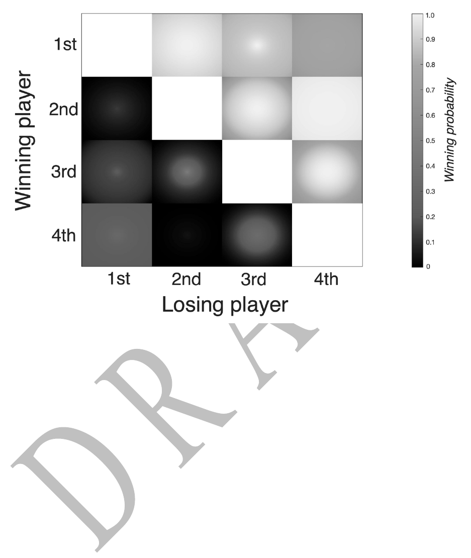
Figure 2

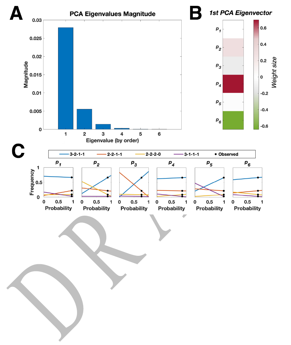
Figure 3

Figure 4