
ISSN: 1962-5361
Disclaimer: This Philadelphia Fed working paper represents preliminary research that is being circulated for discussion purposes. The views
expressed in these papers are solely those of the authors and do not necessarily reflect the views of the Federal Reserve Bank of
Philadelphia or the Federal Reserve System. Any errors or omissions are the responsibility of the authors. Philadelphia Fed working papers
are free to download at: https://philadelphiafed.org/research-and-data/publications/working-papers.
Working Papers
From Incurred Loss to Current
Expected Credit Loss (CECL):
A Forensic Analysis of the Allowance
for Loan Losses in Unconditionally
Cancelable Credit Card Portfolios
José J. Canals-Cerdá
Federal Reserve Bank of Philadelphia Supervision, Regulation, and Credit Department
WP 20-09
February 2020
https://doi.org/10.21799/frbp.wp.2020.09

1
From Incurred Loss to Current Expected Credit Loss (CECL):
A Forensic Analysis of the Allowance for Loan Losses in
Unconditionally Cancelable Credit Card Portfolios
José J. Canals-Cerdá
1
February 2020
Abstract
The Current Expected Credit Loss (CECL) framework represents a new approach for calculating the allowance
for credit losses. Credit cards are the most common form of revolving consumer credit and are likely to present
conceptual and modeling challenges during CECL implementation. We look back at nine years of account-level
credit card data, starting with 2008, over a time period encompassing the bulk of the Great Recession as well
as several years of economic recovery. We analyze the performance of the CECL framework under plausible
assumptions about allocations of future payments to existing credit card loans, a key implementation element.
Our analysis focuses on three major themes: defaults, balances, and credit loss. Our analysis indicates that
allowances are significantly impacted by specific payment allocation assumptions as well as downturn
economic conditions. We also compare projected allowances with realized credit losses and observe a
significant divergence resulting from the revolving nature of credit card portfolios. We extend our analysis
across segments of the portfolio with different risk profiles. Interestingly, less risky segments of the portfolio
are proportionally more impacted by specific payment assumptions and downturn economic conditions. We
also analyze the impact of macroeconomic forecast error and find that it can be substantial and can be impacted
by CECL implementation design features. Overall, our findings suggest that the effect of the new allowance
framework on a specific credit card portfolio will depend critically on its risk profile. Thus, our findings should
be interpreted qualitatively, rather than quantitatively. Finally, the goal is to gain a better understanding of the
sensitivity of allowances to plausible variations in assumptions about the allocation of future payments to
present credit card loans. Thus, we do not offer specific best practice guidance.
Keywords: expected credit losses, allowances, unconditionally cancellable, revolving credit, credit loss
JEL Classification Codes: G21, G28, M41
1
Corresponding author: José J. Canals-Cerdá, Federal Reserve Bank of Philadelphia, Ten Independence Mall,
Philadelphia, PA 19106; 215-574-4127, Fax: 215-574-4146, email: jose.canals-cerda@phil.frb.org
. Special thanks to
Onesime Epouhe and Piu Banerjee for their contributions at an early stage of this research project. The paper has benefited
from conversations with Tom C. Stark about the Survey of Professional Forecasters and from comments received from
Fang Du (Board of Governors of the Federal Reserve System), Chris Henderson (Philadelphia Fed), Arthur Fliegelman
(Office of Financial Research) and two anonymous referees. Any errors or omissions are the author’s.
This paper supersedes “From Incurred Loss to Current Expected Credit Loss (CECL): A Forensic Analysis of the
Allowance for Loan Losses in Unconditionally Cancelable Credit Card Portfolios” by José J. Canals-Cerdá, Federal
Reserve Bank of Philadelphia Working Paper 19-08, January 2019.
Disclaimer: This Philadelphia Fed working paper represents preliminary research that is being circulated for discussion
purposes. The views expressed in these papers are solely those of the authors and do not necessarily reflect the views of
the Federal Reserve Bank of Philadelphia or the Federal Reserve System. Any errors or omissions are the responsibility of
the authors. No statements here should be treated as legal advice. Philadelphia Fed working papers are free to download at
https://philadelphiafed.org/research-and-data/publications/working-papers.
2
Contents
I. Introduction ..................................................................................................................................................................... 3
II. Data and Descriptive Analysis .................................................................................................................................. 7
Data Source ............................................................................................................................................................................ 7
Data Segmentation ............................................................................................................................................................. 8
Historical Charge-Off Performance of Credit Cards ................................................................................................ 9
III. Credit Cards as Unconditionally Cancelable Accounts Under CECL ....................................................... 10
Treatment of Unconditionally Cancelable Accounts Under FASB ASU 2016-13 ........................................ 11
Methodological Challenges: Defining Life of the Loan, Default, and Exposure at Default Under CECL
.................................................................................................................................................................................................. 12
Tracking Credit Card Accounts Performance, Some Stylized Examples ........................................................ 14
IV. Tracking Default, Balance, Exposure at Default, and Loss .......................................................................... 16
Tracking the Evolution of Defaults over Time and Across Cohorts ................................................................. 17
Tracking the Evolution of Balances over Time and Across Cohorts ................................................................ 20
Tracking Loan Loss and the Coverage Ratio over Time and Across Cohorts ............................................... 22
Assessing the Potential Impact of Macroeconomic Forecast Error…………………………………………………23
V. Conclusions..................................................................................................................................................................... 27
VI. Tables and Figures ...................................................................................................................................................... 30
VII. References ....................................................................................................................................................................... 46

3
I. Introduction
The current allowance for loan and lease losses (ALLL) under U.S. generally accepted accounting
principles is an “incurred loss” accounting methodology. Under this methodology, the allowance is a
valuation reserve established and maintained to cover losses that are probable and estimable as of
the reserve calculation date. The methodology has been in place for about 40 years. During the 2008
global financial crisis, however, the existing reserving methodology delayed the recognition of credit
losses on loans and resulted in loan loss reserves that were not adequate. Postcrisis, the Financial
Accounting Standards Board (FASB) considered enhancing standards on valuation and loan loss
provisioning. In June 2016, the accounting standard-setters issued an accounting standards update
(ASU 2016-13) — and the Current Expected Credit Loss Framework (CECL) was born. The new
accounting standard is slated to become effective in 2020, with early adoption permissible in 2019.
2
CECL represents an alternative framework for calculating the allowance for credit losses.
Conceptually, CECL differs from the existing incurred-loss methodology in many respects. CECL is
built on the notion of forward-looking estimated “expected losses.” The measurement of expected
credit losses is based on relevant information about past events, including historical experience,
current conditions, and reasonable and supportable forecasts that affect the collectability of loans.
Also embedded in CECL is the “life of loan” concept. Institutions are expected to reserve for lifetime
losses on loans at the time the loans are originated. The accounting standards update does not
prescribe a specific modeling approach.
Credit cards are revolving accounts for which the user is not required to pay the entire
balance at the end of the cycle. The cardholder can carry a revolving balance, which accrues interest
at the end of each cycle. Credit card portfolios represent a significant contributor to the balance sheet
of many large banks, with some banks specializing primarily in credit card lending. During the 2019
stress test, the Federal Reserve projected overall losses of $410 billion for the 18 participant firms
under the severely adverse scenario. Credit card losses contributed $107 billion, or 26%, to overall
losses, and first mortgage portfolios contributed $14 billion, or 3.4%, to overall losses. The unsecured
and revolving nature of credit card lending are significant factors behind the disproportionate
contribution of credit card losses to overall stress losses.
3
2
Banking regulators have issued Implementation and transition guidance. See the Board of Governors of the
Federal Reserve System (BOG), May 2018, BOG, June 2016, and BOG “Frequently Asked Questions on the New
Accounting Standard on Financial Instruments – Credit Losses.”
3
BOG, June 2019.

4
ASU 2016-13 explicitly addresses the application of CECL to unconditionally cancelable loan
commitments, credit cards in particular.
4
Specifically, ASU 2016-13 indicates that reserves on credit
card portfolios need to be established over the remaining lives of the funded credit card loans (i.e., for
balance on books); reserves need not be established for any additional draws on credit line over the
life of a loan.
The new standard represents a significant departure from current practices under the
existing standards. Implementing the “life of loan” concept underlying CECL may be a significant
challenge for revolving retail products such as credit cards.
Our analysis is descriptive in nature and takes advantage of a rich data set of credit card
accounts that contains relevant information on account characteristics, performance, and payment
behavior. The data set was constructed from individual monthly data submissions to regulatory
agencies from the largest U.S. banks with sizable credit card portfolios. The data set tracks more than
nine years of credit card data, starting with the first quarter of 2008 and continuing up to the second
quarter of 2017. The data set is not meant to represent a specific credit card portfolio of a particular
bank or group of banks.
CECL specifies that reserves need to be established over the remaining lives of the funded
credit card loans, which will depend critically on the stream of future monthly payments. Thus, a
critical component of the analysis of allowances for unconditionally cancelable credit card accounts
under CECL is the specification of payment allocation rules on the remainder of the account balance
at measurement date, or month 0, for as long as the balance remains positive, or until the time of
account default. Payments could be allocated, for example, to incurred finance costs, account balance
at month 0, or debt incurred on any given month as a result of the revolving nature of credit card
lending.
In this paper, we analyze two payment allocation rules that could be interpreted as limit
examples of payment allocation rules, with alternative payment allocation rules likely falling within
these two options. The first payment rule considered allocates all future monthly payments, after
finance charges, to the remainder of the initial reference month 0 balance. We call this the first-in-
first-out (FIFO) allocation rule. A second payment allocation rule, which we call last-in-first-out, or
LIFO, assumes that all future payments, net of finance charges and any incurred expenses, will be
applied to the remainder of month 0 balance for as long as it remains positive or until the time of
4
ASU 2016-13, example 10 states: “Bank M estimates the expected credit losses over the remaining lives of the
funded credit card loans … Bank M does not record an allowance for unfunded commitments on the unfunded
credit cards because it has the ability to unconditionally cancel the available lines of credit.”

5
account default. Thus, in contrast with FIFO, in this second case we are also netting any additional
incurred expenses after month 0 out of monthly payments before applying the remaining payment
to the remainder of month 0 balance.
The non-prescriptive nature of the CECL framework allows for a variety of quantification
methodologies.
5
FIFO and LIFO may be interpretable as boundary payment allocation strategies
under CECL, with LIFO generating higher or equal life of the loan and projected loss estimates.
Lifetime loss on a credit card account will be at least as large as the loan loss projected under CECL
because loss from a defaulted account is likely to include loss resulting from additional draws on its
credit line over the life of the account. Recent industry discussion on the empirical application of the
CECL framework to credit cards has placed some emphasis on the potential implications of the Credit
Card Accountability Responsibility and Disclosure (Credit Card) Act for the allocation of payments
under CECL. Specifically, Section 104 of the Credit Card Act requires that firms allocate any payment
above the minimum periodic payment to the balance with the highest annual percentage rate (APR).
The data available to us for this study are not sufficiently granular to allow for a deep dive into this
question.
The relationship between the payment allocation under the Credit Card Act and the FIFO or
LIFO payment allocation strategies is likely to be complex and endogenous. For example, payment
allocations under the Credit Card Act for a credit card loan subject to a 0 percent promotional interest
rate will be similar to LIFO over the duration of the promotional offer because other payments will
take precedent and a loan subject to this promotional rate will be paid last. Promotional rates are
intertwined with borrowers’ behavior and lenders’ decisions regarding portfolio growth, risk
appetite, and past, current, and expected future economic conditions, among other factors that may
play a role. Different APRs may also be applied to purchases, balance transfers, or cash advances, for
5
This topic has been addressed in recent memos of the Financial Accounting Standards Board (FASB)’s Transition
Resource Group (TRG) for Credit Losses, a task force within the FASB tasked with the job of “solicit, analyze, and
discuss stakeholder issues arising from implementation of the new guidance.” Specifically, Memo No. 5:
“Determining the Estimated Life of a Credit Card Receivable”; Memo No. 5A: “Determining the Estimated Life of a
Credit Card Receivable — Appendix A”; Memo No. 6: June 2017 “Meeting — Summary of Issues Discussed and
Next Steps”; Memo No. 6B: “Addendum to Memo No. 6 — Determining the Estimated Life of a Credit Card
Receivable.” In particular, Memo No. 6B indicates “entities are not limited to the payment determination and
allocation methodologies discussed in the June 12, 2017 TRG meeting and October 4, 2017 Board meeting if other
appropriate means of estimating the expected life of a credit card receivable are available.”
https://www.fasb.org/jsp/FASB/Page/SectionPage&cid=1176168064117.

6
example. Incidentally, a penalty APR usually applies to delinquent accounts. Thus, the Credit Card Act
if applied to CECL may increase implementation costs.
6
It is not our objective to highlight any specific payment allocation proposals currently being
discussed among interested parties. Also, given the principle-based nature of the CECL framework, it
is also not our objective to offer specific best practice guidance. Instead, we believe that there is value
in conducting an analysis of the impact of explicit and transparent payment allocation rules looking
back at historical data across relevant risk segments of a portfolio, which is our primary objective.
Thus, our analysis should not be regarded as endorsement of any specific payment allocation rule.
Our analysis relies on the construction of a synthetic portfolio of credit card accounts. The
primary data in our analysis consist of monthly submissions of detailed account level credit card data
from large banks collected by regulatory agencies. We analyze the performance of allowances at the
overall aggregated portfolio level as well as across segments of the portfolio properly differentiated
by their level of credit risk. We analyze the behavior of different measures of allowances across
cohorts, starting with the first quarter of 2008 and up to the second quarter of 2017. We track the
performance of each account in our sample for at least five years (and up to nine years) from each
reference month, or up to the time of account’s closure or default. Our period of analysis encompasses
a variety of economic conditions, including the bulk of the Great Recession and the subsequent
recovery.
We focus our analysis, both at the portfolio level and across risk segments, on three major
themes: defaults, balances, and credit loss. The specification of a payment allocation rule under CECL
plays a significant role in the definition of loan default. In general, risk profile is the primary
determinant of default at the segment level, but the impact of the specific payment allocation rule
considered is also significant. The divergence in cumulative default curves across payment allocation
rules considered is relatively small over the initial projection months and increases significantly after
that. Differences across payment allocation rules are, proportionally, more pronounced for less risky
segments. Thus, a portfolio’s risk composition is likely to play a significant role on the final CECL
impact of any specific payment allocation rule. Across payment allocation rules, projected default
rates increased significantly during the downturn and then experienced a significant decrease as
economic conditions improved.
6
TRG staff raised some concerns with the level of complexity introduced by the Credit Card Act (referred as View B
in the memo). Specifically (Memo No. 6B), “The staff notes that while this may be an operable method to apply
View B, it would be a new concept of the estimate of credit losses that credit card issuers would need to develop,
which may increase implementation costs.” “The staff also notes that if View B were to be required it may affect
flexibility and scalability for smaller institutions that may not currently have the resources to apply the approach
under View B.”
7
We also observe significant differences in the evolution of the remainder of month 0 balances
across payment allocation rules and in relation to the evolution of account balances. The observed
differences in the evolution of balances across different payment allocation rules have important
implications for the evolution of loan default and loan loss at default.
Projected allowances are significantly higher during the period of the economic downturn.
Perhaps contrary to intuition, our analysis suggests that low-risk segments, and portfolios, are
proportionally likely to be most sensitive to specific assumptions about payment allocation rules, and
differences across payment allocation rules increase during the downturn. These findings also
suggest that portfolios with different levels of credit risk are likely to experience dissimilar impacts.
Thus, our findings should be interpreted from a qualitative, rather than quantitative, perspective.
Last, we highlight how projected allowances differ significantly from realized credit loss. This is
primarily because of the focus of CECL on the concept of credit card loans at observation time, which
contrasts with the revolving nature of credit card lending. In our empirical analysis, we also address
the issue of sensitivity of CECL projections to macroeconomic forecasting error and observe that the
impact can be significant.
In the next section, we present the data and conduct a descriptive statistical analysis. In
Section III, we analyze in detail the treatment of unconditionally cancelable accounts under FASB ASU
2016-13. In Section IV, we present relevant empirical findings. In Section V, we present conclusions.
Tables and figures are presented in a separate section at the end of the paper.
II. Data and Descriptive Analysis
Data Source
Our analysis employs a sample of credit card accounts from a data set that combines credit card
portfolios from some of the largest U.S. banks with significant credit card exposures. The original data
comprise monthly account characteristics and performance information from the first quarter of
2008 and up to the second quarter of 2017, or up to the time the account is closed or charged off. The
data contain more than 100 variables that provide monthly observations of the credit card

8
characteristics; credit attributes of the cardholders such as credit score, payment, and usage
behavior; and delinquency status for each individual account.
7
The data were primarily collected with the objective of conducting supervisory work,
including the annual stress test exercise. Because of the confidentiality of the data, all the information
provided in this paper is reported at a highly aggregated level. Our sample is neither meant to be
representative of the overall credit card lending market nor representative of the credit card
portfolio of any particular bank or group of banks. However, our analysis is meant to offer helpful
qualitative insights about the loss performance of credit card portfolios across risk segments under
different economic conditions.
Data Segmentation
Our analysis is primarily descriptive and conducted at the segment level for a group of segments
derived from account-level information on credit score, historical payment, and usage behavior as
well as delinquency status.
Table 1 describes the segmentation variables considered and the different segments
generated by combining these variables. Specifically, we consider nine different segments of
accounts: dormant accounts, transactor accounts with a 0 balance, transactor accounts with positive
balance, three segments of revolver accounts by risk score ranges, and three segments of delinquent
accounts by severity of delinquency. From our interpretation of ASU 2016-13, dormant accounts and
transactor accounts with a 0 balance at observation time will not require an allowance.
8
Thus, our
primary focus will be on these seven segments that will require an allowance under CECL.
Table 2 provides a very preliminary view of the risk across different segments considered by
reporting average sample default rates over different time horizons. The table reports significant
differences in risk profile across segments even in our simple segmentation framework. Dormant and
transactor accounts exhibit very low default risk even over a five-year time horizon. In contrast,
revolver accounts are significantly more risky, and we can further differentiate risk by combining
7
These submissions are commonly known as FR Y-14M reports and consist of Domestic First Lien Closed-End 1-4
Family Residential Loan, Domestic Home Equity Loan, and Domestic Credit Card data collections. A link to available
public information about the data is included in the References section.
8
ASU 2016-13 indicates that reserves on credit card portfolios need to be established over the remaining lives of
the funded credit card loans.

9
revolver status with credit scores. Not surprisingly, delinquent accounts have the highest risk of
default. In future sections, we provide additional analysis of risk across segments.
Historical Charge-Off Performance of Credit Cards
Figure 1 provides additional intuition about the level of risk embedded in the credit card portfolios.
The figure provides strong evidence of the relationship between credit card charge-off rates and
economic conditions. Furthermore, the severity and duration of elevated charge-off rates seem to
track well the severity and duration of recessions and increases in unemployment rate.
9
Figure 2 presents median recovery rates across banks and over the time period of our
analysis. Recovery rates measure the percentage of gross charge-off that is recovered. The figure also
includes median 12- and 24-month net charge-off rates for the same group of banks defined as the
sum of 12 months and 24 months net charge-offs as a percentage of portfolio balance. The net charge-
off rates presented in this figure are broadly consistent with those presented in Figure 1, which are
representative of a larger sample of banks. The figure also indicates that recovery rates, as a
percentage of charge-offs, were at their lowest point around the same time as charge-off rates were
at their highest.
Figures 1 and 2 highlight the significant increase in net charge-offs over the economic
downturn, as a result of an increase gross charge-offs and a decrease in recovery rates. Thus, a focus
on the dynamics of gross charge-offs primarily will not provide a sufficiently stressed view of the
impact of economic downturns on net portfolio loss. On the other hand, an analysis of net charge-offs
requires potentially judgmental assumptions about the timing and allocation of recoveries from
defaulted accounts, which are not usually tracked at the account level in credit card portfolios.
With the wisdom of hindsight, Figure 3 provides a window into the performance of the
existing allowance framework during the recent financial crisis. These results are derived from bank-
specific information that we don’t report for confidentiality reasons. The figure displays median
portfolio allowances and 12-month cumulative charge-offs, as a percentage of assets, as well as the
median coverage rate defined as the number of months of forward-looking net charge-off losses that
can be sustained by contemporaneous allowance levels.
The 12-month forward-looking, cumulative median charge-off rate picked around 2009 in
our portfolio and remained elevated well into 2011. The allowance rate increased significantly from
9
Canals-Cerdá and Kerr (2015) conduct a comprehensive study of the relationship between unemployment and
the risk of credit card portfolios. See also Banerjee and Canals-Cerdá (2013).
10
2008 to 2010 and decreased after that in conjunction with a significant, and continued, decrease in
charge-off rates that began around 2010. Thus, the pick up in allowances lagged behind the pick up
in forward-looking cumulative charge-off rates by about a year, or longer. The median coverage rate
was significantly below average in 2008, experienced a steep and continued increase between 2008
and 2010, and extended its increase into 2011, after which it began a continued decline, stabilizing
at around the nine to 11 months median coverage rate range. The behavior displayed by the
allowance rate and coverage rate in Figure 3 is in line with the common view that the “incurred loss”
accounting methodology, employed by bank holding companies over the past 40 years, delayed the
recognition of credit losses during the 2008 global financial crisis and resulted in loan loss reserves
that were not adequate for the level of stress during the downturn.
III. Credit Cards as Unconditionally Cancelable Accounts Under CECL
The special treatment of credit card portfolios under ASU 2016-13 requires us to revisit the
traditional framework of analysis of expected loss and credit risk in revolving accounts. The ASU
2016-13 update describes unconditionally cancelable accounts as those in which the unfunded
portion of a line of credit may be unconditionally canceled at any time. In most cases, credit card
accounts will fall into this category.
It is standard industry practice to analyze expected credit card loss as a function of three
components: the probability of default, the exposure at default, and the loss given default, with
expected loss defined as the product of these three factors. For revolving accounts in particular, the
analysis is not constrained by the amount of the debt carried at observation time. However, the
account balance at observation time is usually regarded as an important driver of default and future
expected loss in the case of default. Generally, the expectation is that a borrower at risk of default is
likely to increase her level of borrowing prior to default. Thus, the standard quantitative analysis of
exposure at default is not bounded by the account balance at observation time.
In this section, we look closely at the treatment of credit card accounts under ASU 2016-13.
First, we review the concept of an unconditionally cancelable account under CECL; second, we
consider conceptual and methodological challenges brought about by this framework, such as life of
loan or the concept of default and exposure at default under CECL; and finally, we consider the
implications of different assumptions about the treatment of future payments and illustrate these
concepts with highly stylized numerical examples.

11
Treatment of Unconditionally Cancelable Accounts Under FASB ASU 2016-13
For unconditionally cancelable accounts, ASU 2016-13 stipulates that banks would “estimate the
expected credit losses over the remaining lives of the funded credit card loans.” It also specifies that
“even though Bank M has had a past practice of extending credit on credit cards before it has detected
a borrower’s default event, it does not have a present contractual obligation to extend credit.” Based
on that reasoning, it also indicates that “an allowance for unfunded commitments should not be
established because credit risk on commitments that are unconditionally cancellable by the issuer
are not considered to be a liability.”
10
The FASB statements referred to in the previous paragraph have significant implications for
the analysis of allowances. For starters, they specify that there should not be an allowance for
unfunded commitments.
Typical credit card segments of accounts that entirely fall in this category of unfunded
commitments are dormant accounts (i.e., accounts with no balance and no financial activity), and
transactor accounts that don’t carry a balance in a particular month.
11
Thus, dormant accounts and
transactor accounts that don’t carry a balance in a particular month will not necessitate an allowance
under CECL. These segments of accounts represent a large percentage of accounts in the typical cards
portfolio.
Similarly, unfunded commitments of credit card accounts with positive utilization are also
not considered a liability under CECL. Thus, an account’s exposure at default under the CECL
framework will not be larger than its present funded commitment. This represents a key distinction
with respect to traditional risk quantification frameworks, such as the Basel advanced approaches
framework, typical stress-testing frameworks, and similar standard approaches for quantifying
credit risk. Generally, the expectation is that a borrower at risk of default will likely continue to draw
from an available line of credit prior to default, and risk models are designed to account for this
empirical regularity.
10
See FASB, ASU 2016-13, p. 138.
11
Transactor accounts are usually referred to as accounts that carry no debt from month to month and incur no
finance charges.
`

12
Methodological Challenges: Defining Life of the Loan, Default, and Exposure at Default Under CECL
A recently publicly circulated FASB memo offers additional information about the analysis of
allowances for unconditionally cancelable accounts under CECL.
12
The memo didn’t reach any firm
conclusion, but it provided a window into the conceptual and methodological challenges firms may
face in the process of implementing CECL and perspectives into the type of preliminary analysis being
conducted by stakeholders in this area. The memo focuses specifically on the estimation of the life of
a credit card receivable. The memo points out “estimating the remaining life of a credit card
receivable balance is dependent on estimating the amount and timing of the payments expected to
be collected on it.” In contrast with closed-end loans, estimating the life of a credit card receivable
balance “is significantly more complex because in addition to future expected payments there also
will be new borrowing activity over the remaining life of the measurement date balance.”
It is not our objective to analyze specific proposals currently being discussed in the industry.
Instead, we believe there is value in conducting an analysis of the impact of different plausible
payment allocation rules looking back at historical data at different points in time and across risk
segments of a portfolio.
In our data, we observe a rich set of account characteristics and historical account
performance. We also observe monthly account balances, payments, and overall finance charges at
the account level.
13
With this information in hand, we can analyze how different types of plausible
assumptions about allocations of the future stream of payments impact the forecast of balance, life
of the loan, the risk of loan default, and loss at the time of loan default, and ultimately, how they
impact current expected credit loss on the funded credit card loans at the portfolio, or segment, level.
Specifically, in the next paragraphs, we analyze two possible stylized ways of accounting for future
payments, or payment rules. In our view, these two payment allocation rules could be interpreted as
limit examples of payment allocation rules, with alternative plausible payment allocation rules likely
falling within these two options.
A first approach, which we call first-in-first-out, or FIFO, assumes that all future payments,
net of finance charges, will be applied to the remainder of the balance existing at the measurement
date, or month 0, for as long as the balance remains positive or until the time of account default. The
12
See FASB Memo No. 5, June 2017.
13
Banks have access to all individual card transactions and detailed information on payments, promotions, interest
rates, and finance charges; our data are not as granular in this regard.
13
minimum number of months until the remainder of month 0 balance equals zero or default occurs
will represent the life of the loan in this case.
A second approach, which we call last-in-first-out, or LIFO, assumes that all future payments,
net of finance charges and any incurred expenses, will be applied to the remainder of month 0 balance
for as long as it remains positive or until the time of account default. The minimum number of months
until one of these events occur will represent the life of the loan in this case. Under LIFO, a payment
to the remainder of the balance will not occur before all incurred finance charges and incurred
expenses have been paid off. Thus, the remainder of month 0 balance will be reduced in a future
month only if the actual monthly revolving balance falls below the rolling remainder of month 0
balance (i.e., the last incurred finance charges and incurred expenses will be paid off first). Thus, at
any future time t, the remainder balance will be the minimum of the remainder of month 0 balance
and the stream of revolving monthly balances up to that point. In the next paragraphs, we provide
additional detail about FIFO and LIFO, and in the next subsection, we analyze some examples,
including actual examples of account behavior observed in our data as well as stylized numerical
examples.
The main difference between FIFO and LIFO is that, in the case of LIFO, in addition to finance
charges registered at the time of the monthly payment, we also deduct from monthly payments any
incurred expenses registered at the time the payment is due, before subtracting the residual payment
from the remainder of the balance at month 0.
The FIFO and LIFO concepts can be expressed analytically after introducing some necessary
notation. Denote by
0
the account’s balance existing at month 0 and more generally denote by
the account’s balance existing at month t; denote the payment in month t, net of finance charges, as
and denote the remainder of month 0 balance t months into the future as
0
(
)
.
Under the FIFO assumption, the remainder of month 0 balance at time t = 1 can be computed
as,
0
(
= 1
)
=
(
0
−
1
, 0
)
,
and the remainder of month 0 balance at any future time t+1 can be computed as,
0
(
+ 1
)
=
(
0
(
)
−
+1
, 0
)
.
Under the LIFO assumption, the remainder of month 0 balance at time t = 1 can be computed
as,
14
0
(
= 1
)
=
(
0
,
1
)
,
with
1
representing the account’s balance one month after the reference month 0. Similarly, the
remainder of month 0 balance at month t +1 after the reference month 0 can be computed as,
0
(
+ 1
)
=
(
0
(
)
,
+1
)
,
with
representing the account’s balance t months after the reference month 0.
Observe that under LIFO, the remainder of the month 0 balance at month t+1 equals the
minimum balance attained by the account during the period [0,t+1] (i.e., the remainder of the month
0 balance will equal the revolving balance in a particular month when the revolving balance falls
below the remainder of month 0 balance until that point). The remainder of the month 0 balance will
be equal to 0 when the revolving balance in a particular month becomes 0 for the first time, at which
point it is assumed that the loan will have been repaid.
Under both concepts, the remainder of the month 0 balance will be fully paid at month when
the remainder of the month 0 balance reaches a value of 0 balance,
0
(
)
= 0 <
0
(
− 1
)
,
with representing the life of the credit card loan in this case.
A credit card account is at risk of default as long as it remains open, but a loan incurred in
month 0 is at risk of default only while it is being repaid (i.e., during the length of the life of the loan).
If an account defaults at time t before the remaining balance reaches value 0 (i.e., before the
end of the life of the loan), then we consider that the loan is in default in an amount equal to the
remainder of month 0 balance, i.e.,
0
(
)
.
Tracking Credit Card Accounts Performance, Some Stylized Examples
Table 3 presents three stylized examples that illustrate the concepts described previously. For
simplicity, we don’t explicitly consider finance charges. The first example presents the case of a credit
card loan in which the account receives monthly payments and there are no additional charges after
month 0. In this case, the FIFO and LIFO concepts produce exactly the same outcomes. This is
generally the case when the account incurs no additional charges after month 0.
15
In our second example, the account incurs new monthly charges and receives monthly
payments that are not large enough to compensate for monthly charges (i.e., the account balance
continues to grow after month 0). In this case, the LIFO life of the loan will go beyond the 12 months
that are being tracked in this table, and the LIFO remainder balance will stay constant over the entire
tracking period. In contrast, the FIFO life of the loan will be equal to 10 months, and the path of the
remainder balance will be remarkably different from the LIFO case.
In the last example, the account charges and payments over the next 12 months will generate
different paths for the remainder of the balance and the life of loan under LIFO and FIFO. But in both
cases, the remainder balance will be 0 before the end of the tracking period, while the actual account
balance will drop to 0 at month 7 but will end up growing significantly by the end of the tracking
period.
Each of the previous three examples considers the case in which the account does not default
over the period of analysis. If instead we assume that the account defaults in month 6, for example,
then the FIFO remainder loan exposure at default will be equal to 40, 40 and 0, for examples 1 to 3,
in the case of FIFO (i.e., no loan default in the last case), while the remainder loan exposure at default
will be equal to 40, 100 and 40, for examples 1 to 3, under LIFO.
In Figure 4, we track the evolution of a few selected accounts in our data starting at a fixed
initial date, or month 0, and with reported amounts normalized with respect to the account’s balance
at that initial date. We track balances and payments as well as three different measures of remainder
balances after month 0. The selected examples provide insights about the impact of different
payment allocation rules.
In Figure 4.a, the different payment allocation rules considered result in an almost identical
path across the remainder of month 0 balances, until month 24, at which point the remainder of the
month 0 balance is completely paid off. Thus, the life of the loan is 24 months in this case under both
FIFO and LIFO. After month 25, the tracked revolving account balance increases because of an
increase in monthly borrowing with respect to monthly payments. In Figure 4.b, we observe a
divergence between the two measures of the remainder of the month 0 balance. Under FIFO, the life
of the loan is 15 months, while under LIFO, the life of the loan is 32 months. Between months 15 and
32, the remainder of the month 0 balance exposed under LIFO is about 40% of the balance at time 0.
Figure 4.c depicts an account for which balances increase significantly after month 0, while monthly
payments are comparatively low. In this instance, under FIFO, the life of the loan is equal to 25
16
months, while under LIFO, the remainder of the month 0 balance remains constant at 100% of the
initial balance at the month 0 over the tracked 37-month period.
Figures 4.d to 4.f represent examples of accounts for which the final outcome prior to month
37 was account default, but not in all cases did this account default result in loan default. In all three
cases, the final default balance was significantly larger than the initial balance at month 0, something
that is not atypical when a credit card defaults. The main difference among these three examples is
in the remainder of the month 0 balance at the time of the account default. In example 4.f, the
remainder of the month 0 balance becomes 0 at month 5, while the account does not default until
month 33 (i.e., this case will not be categorized as a loan default even though the account eventually
ends up defaulting). In the case of Figure 4.e, the remainder of the month 0 balance will be positive
at the time of account default, under both payment allocation rules considered (i.e., we will record a
loan default in this case). In this case, the loan exposure at default will be close to 100% of the balance
in the case of LIFO, while it will be close to 30% of the balance under FIFO. In Figure 4.d, the
remainder of the month 0 balance at the time of account default will be positive under LIFO, while it
will be 0 under FIFO. In this case, we will be recording a loan default under LIFO and recording a loan
paid off under FIFO. In all cases considered in which the final outcome is account default over the
tracking period, the remainder balance at default under FIFO and LIFO is either 0 or significantly
lower than the observed account balance at default.
IV. Tracking Default, Balance, Exposure at Default, and Loss
A key aspect of the CECL implementation for credit cards is the allocation of future payments to the
remainder balances after month 0. The adoption of a specific payment allocation rule will determine
the life of the loan at the account level, the evolution of remainder balances after month 0, and the
default and loss experienced after month 0 for CECL purposes. More important, the specific payment
allocation rule implemented will determine, along with the historical experience, the projection of
portfolio allowances under CECL for any specified economic forecast.
In the next paragraphs, we analyze, at the portfolio level and for specific segments, the
evolution of default, balances, and loss, from an initial predetermined starting point in time or “month
0.” The FIFO and LIFO payment allocation rules defined in the previous section will be applied at the
account level and, after aggregation at the portfolio or segment of accounts, will determine default
rates, balance rates, and loss rates that can be projected forward from a predetermined starting point
in time, or month 0.
17
The portfolio employed in our analysis was not constructed to be representative of the overall
credit card industry. Even an industry representative portfolio cannot be expected to provide precise
guidance on the impact of CECL at any specific institution given the heterogeneity of portfolios and
strategies prevalent across credit card lenders. Thus, instead of focusing on a specific representative
portfolio, we present descriptive information across the characteristic risk segments defined in Table
1. Our analysis of segments of revolver accounts with different levels of risk as well as our analysis
of segments of delinquent accounts by severity will provide relevant insights on the performance of
credit card portfolios with different risk distributions.
We focus our attention on a few selected segments by risk profile; considering all segments
would overcomplicate our exposition. Pure dormant and transactors with a 0 balance don’t require
an allowance under CECL because they don’t carry a balance as of month 0. Furthermore, transactor
accounts with a positive balance have a very low probability of default over the short and medium
term, as evident in Table 2, and will carry a small allowance irrespective of the payment rule that
emerges as common industry practice and should be generally marginally sensitive to the choice of
payment allocation rule. Thus, we focus our attention primarily on the revolver and delinquent
segments. For revolvers, we focus on the low-risk and high-risk segments, with the elevated risk
segment in our experience behaving in an intermediate way between these other two segments
considered. For the delinquent case, using our own judgment, we will present at times results
aggregated for the overall delinquency segment; at other times, we will present separate results for
low-delinquency, elevated-delinquency, and high-delinquency segments.
Tracking the Evolution of Defaults over Time and Across Cohorts
This subsection documents the differences between cumulative default curves across payment
allocation rules and with respect to traditional cumulative default curves at the account level. A credit
card account is at risk of default as long as it remains open, but a credit card loan at reference month
0 is at risk of default only while it is being repaid (i.e., during the life of the loan). Differences in
cumulative default curves across payment allocation rules are driven by differences in the life of the
loan associated with differences in the evolution of the remainder of the month 0 balances, as
illustrated in the previous section. For the same reason, we can anticipate differences in the evolution
of balances and losses across payment allocation rules; these will be discussed in the subsequent
subsections.
Figure 5 presents Kaplan-Meier (K-M) cumulative default curves derived from the
implementation of the FIFO and LIFO payment allocation rules (i.e., tracking loan defaults), along

18
with the more traditional cumulative default curves at the account level. The Kaplan-Meier estimator
represents a standard nonparametric technique for estimating the probability of survival, or in our
case, the cumulative default probability, across time for a time-related event, like default.
14
We
present results at the portfolio level and for three different segments: the low- and high-risk revolver
segments and the segment of delinquent accounts. We present results aggregated across cohorts
because the patterns observed in the data are similar for different cohorts, but with the expected
variations in severity among the cohorts more directly impacted by the downturn.
Figure 5.a presents results at the portfolio level. The figure reveals three main patterns in the
data. First, the choice of payment allocation rule plays a significant role in the definition of default.
We observe a substantial divergence between the FIFO and LIFO K-M cumulative default curves, with
a significant divergence starting around month 20. Second, perhaps not surprisingly, the divergence
in cumulative default curves is relatively small over the initial 10 months and intensifies after that.
The FIFO K-M curve is the first one to reach a plateau around month 40, while the LIFO curve seems
to reach a plateau around month 80. There is no apparent plateau in the default curve at the account
level, although the slope of the curve decreases over time. Third, there is a clear divergence between
the cumulative default curve at the account level and any of the cumulative loan default curves
considered. This is consistent with our intuition since the life of the account is expected to exceed the
life of the loan in most cases.
Figure 5.b provides additional insights about the evolution of defaults. The figure presents
cumulative default curves for three segments of accounts: the low-risk revolver segment, the high-
risk revolver segment, and the delinquent segment. There is a clear differentiation in cumulative
default curves across segments, which indicates that risk profile is an important determinant of
default and outweighs the importance of the payment allocation rule, at least for the highly
differentiated risk segments considered.
As expected, the more risky segments are associated with steeper cumulative default curves.
For the delinquent segment, most of the defaults occur within the first 10 months and there are no
significant differences across payment allocation rules over this time frame. Significant differences
across payment allocation rules in the delinquent segment emerge after 30 months, but even then,
these differences are proportionally small when compared with other segments. The high-risk
revolver segment follows a similar pattern, but the cumulative default curves are comparatively less
steep and the bulk of defaults are not realized until the 40th month. In this case, there is no apparent
plateau in the cumulative default curves for the account and LIFO curves, while a plateau occurs for
14
See Kaplan and Meier (1958) or Kalbfleisch and Prentice (2002).
19
the FIFO curve around 40 months. Finally, the low-risk revolver segment follows a similar pattern;
however, most defaults occur by the 30th month for the FIFO curve, while defaults continue to
increase after that for the LIFO and account curves.
The insights gained from our analysis of Figure 5.b also contribute to a better understanding
of the portfolio-level dynamics observed in Figure 5.a. Delinquent accounts, as well as accounts in
high-risk segments contribute a high proportion of defaults during the first 20 months, adding to a
steeper portfolio default curve initially. The less risky segments of accounts increase their
contribution to overall portfolio defaults after the initial months, contributing to a softening in the
slope of the default curve.
Perhaps the most relevant finding from Figure 5.b is the observation that differences across
payment allocation rules are, proportionally, more pronounced for less risky segments. They have a
comparatively lower impact for the high-risk segments, with the lowest impact associated with the
segment of delinquent accounts. In particular, for the low-risk segment, at month 80, the value of the
LIFO curve is about 50% higher than that of the FIFO curve, and the value of the account default curve
is about 100% higher. The differences are proportionally less pronounced for higher-risk segments.
Finally, our findings from Figure 5.b also have important implications for the analysis of the
potential impact of CECL across portfolios with different risk profiles. Specifically, they suggest that
differences in payment allocation rules can have significant impact on the overall cumulative default
curves under CECL. Furthermore, the impact will be dissimilar across segments with different risk
profiles and may be proportionally largest in lower-risk profile segments. Thus, a portfolio’s risk
composition is likely to play a significant role on the final CECL impact of any specific payment
allocation rules.
Figure 6 considers the evolution of default rates over a time frame with a mix of economic
conditions. The figure tracks five-year cumulative default rates across different cohorts. Specifically,
we define the initial reference “month 0” to take values at each quarter between the first quarter of
2008 and the first quarter of 2012; after the initial reference month is fixed, we analyze each cohort’s
default rate over a five-year window and report that five-year default rate in the graph for each
quarterly cohort. From Table 5, we already know that most defaults will occur within the initial 60-
month window, so our focus on the five-year default rate does not represent a significant restriction.
In principle, when computing default rates over a five-year period, we would consider it
reasonable to expect a certain level of default averaging across a five-year window with a mixture of
economic conditions. On the other hand, under the treatment of credit cards as unconditionally
cancelable accounts, the bulk of defaults realized under CECL are likely to occur within the first two

20
years after month 0, as Figure 5 indicates. Furthermore, for credit cards, the difference between the
charge-off in good times versus the charge-off in a downturn can be very significant, as Figure 1
indicates.
15
Figure 6 shows that, with the perfect foresight assumption implicit in our analysis, long-term
default rates experienced an increase in severity between the first quarter of 2008, the first
observation period, and the second quarter of 2009. Default rates were elevated during the overall
downturn period and experienced a significant decline as economic conditions improved. Looking at
Figures 6.b to 6.e, we also observe differences in performance across segments. The more risky
segments are more severely impacted by downturns in absolute value, but it is worthwhile to point
out that the more risky segments are also proportionally (i.e., in terms of percentage change) less
affected by economic fluctuations.
16
Specifically for FIFO, we observe fluctuations in default rate from
bad to good times between 0.06 and 0.03 in the low-risk segment (i.e., a 100% increase), between
0.28 and 0.16 in the high-risk segment (i.e., a 75% increase), and between 0.58 and 0.4 in the
delinquent segment (i.e., a 45% increase).
Default constitutes the critical trigger of credit risk, but another significant contributor to
credit risk is loan exposure at default, particularly for the case of revolving accounts. The next
subsection looks at the evolution of the remainder of the month 0 balance at the portfolio level, across
segments, and under different payment allocation rules. In the final subsection, we combine the
concept of default and the remainder loan exposure at default after month 0 and look closely at the
concept of portfolio credit loss.
Tracking the Evolution of Balances over Time and Across Cohorts
Figures 7 and 8 look at the evolution of portfolio balances across cohorts, across segments, at the
account level, and for different payment allocation rules. Figure 7.a depicts the evolution of balances
across cohorts at the portfolio level and for the segments of transactor, revolver, and delinquent
accounts. Perhaps not surprisingly, revolver accounts consistently carry the largest balances, and
transactor accounts (excluding these with a 0 balance), the smallest. Some readers may find it
surprising that balances for delinquent accounts are generally lower than those of revolver accounts.
This may be the result of the specific composition of our portfolio. More likely, accounts that become
delinquent are primarily associated with lower credit scores and lower credit lines, and thus have
15
Figure 1 also indicates that the downturn was followed by a long period of low credit card charge-off rates.
16
This is consistent with prior research by Canals-Cerdá and Kerr (2015).
21
limited ability to borrow. Finally, we also observe that balances associated with delinquent accounts
seem to be more sensitive to fluctuations in economic conditions. One possible explanation of this
phenomenon is that worse macroeconomic conditions increase the proportion of delinquent
accounts with higher initial credit score, higher credit limits, and higher ability to borrow. Further
study of these issues is warranted but is beyond the scope of our analysis.
Figure 7.b draws the evolution of account balance and the remainder of the month 0 loan
balance for different payment allocation rules. We observe significant differences between the
evolution of account balances and the evolution of the remainder of the month 0 loan balance under
different payment allocation rules. Specifically, 40 months after month 0, only about 10% of the
original balance at month 0 remains under FIFO, while about 20% of the balance remains under LIFO.
In contrast, the revolving portfolio balance after 40 months is about 60% of the original balance. The
attrition in the revolving portfolio balance may be due to account closure, charge-off, account
transitions to transactor or dormant, or the availability of other sources of credit for accounts with
improved credit scores.
Figure 8 looks at the evolution of the remainder of the month 0 balance across segments up
to 48 months into the future at the account level and for different payment allocation rules. We
observe the largest differences in the remainder of the month 0 balance curves for the low-risk
segment of accounts and the smallest differences in the delinquent segments. This indicates that
differences in payment allocation rules are likely to have the largest impact in the low-risk segments.
Low-risk borrowers are likely to contribute higher payments to the remainder of the month 0
balance, thus differences in payment allocation rules are likely to have a larger impact in this
segment, which may help to explain the significant differences. On the other hand, delinquent
borrowers are likely to contribute low or 0 payments to the remainder of the month 0 balance, and
the reduction in segment balance over time are likely the result of defaults. Thus, it should not be
surprising that delinquent segments display the smallest differences across payment allocation rules.
The insights provided by Figure 8 don’t change for specific cohorts; for this reason, we include here
only the results aggregated across cohorts.
The difference in the evolution of balances among payment allocation rules across risk
segments undoubtedly plays a significant role in the evolution of loan default and loss at default
across risk segments and cohorts. In the next subsection, we focus our attention on the analysis of
portfolio credit loss, which combines the effect of different payment allocation rules on default and
the remainder of the month 0 balance at default.

22
Tracking Loan Loss and the Coverage Ratio over Time and Across Cohorts
In this subsection, we analyze current expected credit loss curves after month 0, for specific payment
rules, as well as standard portfolio or segment loss curves, with all the results normalized by the
portfolio or segment balance at month 0. From the perspective of account default and loss, we
consider the account as being at risk of default as long as it remains open. Also, loss at default at the
account level is defined as the account balance at the time of default. The trigger of default is when
the account reaches 150 days past due or the account is charged off for other reasons.
17
Under CECL,
default and loss are measured at the loan level. Specifically, a loan will be at risk of default as long as
it stays open (i.e., as long as the remainder of the month 0 balance is positive). The trigger of default
of an open loan is the same as the trigger of account default. Thus, for our purposes, loan default and
account default occur simultaneously while the loan stays open. When a loan defaults, we define the
gross loan loss as the remainder of the month 0 balance at the time of default. The focus here is on
gross loss; we don’t deal with the problem of allocation of recoveries and net loss.
Figures 9 and 10 analyze the variation in loss curves across cohorts, portfolio segments, and
payment allocation rules. Figures 11 and 12 focus on the analysis of loss coverage under different
payment allocation rules.
Figure 9 looks at the evolution after month 0 of cumulative loss curves across cohorts and for
different payment allocation rules. First, we observe that the cohorts that were more directly
impacted by the last financial crisis exhibit significantly more severe loss curves. The 2008Q1 cohort,
with March 2018 as the associated month 0, exhibits the largest portfolio losses in the long run, but
rank ordering across loss curves is not maintained across payment allocation rules. FIFO, and to a
lesser extent LIFO, curves are highly sensitive to losses over the short and medium term (i.e., losses
occurring over the initial 24-month period), while overall account portfolio losses are more affected
by long-run losses. Figure 9.c reports differences over time in loss curves across payment allocation
rules. The figure shows large differences in loss rates across payment allocation rules, and these
differences are magnified in cohorts more heavily impacted by the economic downturn.
Figure 10 looks at the evolution from month 0 of loss curves for different payment allocation
rules across risk segments: low-risk revolver, high-risk revolver, and delinquent. Consistent with
previous findings, we observe that, proportionally (i.e., in terms of percentage change), the largest
differences across payment allocation rules are associated with the lowest-risk segments.
17
Most banks will freeze or close an account after 90 days past due, while the Basel II framework assumes that
default occurs at 180 days past due. We choose 150 days as the trigger of default to minimize potential problems
of missing data reported by the banks that may arise if a bank moves an account to a collections system.
23
Specifically, for the low-risk revolver segment projected portfolio losses after five years are about
350% of loss under FIFO and about 200% of loss under LIFO. For the high-risk revolver segment
projected portfolio losses after five years are about 200% of loss under FIFO and about 150% of loss
under LIFO. For the delinquent segment losses under FIFO and LIFO after five years are similar and
only about 8% lower than portfolio loss. These observations are relevant for the analysis of specific
payment rules across portfolios with different risk profile distributions.
Figures 11 and 12 focus on the analysis of loss coverage across cohorts, portfolio segments,
and payment allocation rules. The figures include portfolio/segment loss curves across cohorts for
different time spells: 15 months into the future, 18 months, and so on. The figures also depict loss
curves under FIFO/LIFO. The intersection of portfolio/segment loss curves with FIFO/LIFO loss
curves represents the coverage rate under FIFO/LIFO allowances (i.e., a measure of how many future
months of actual portfolio loss are covered by the corresponding allowance). However, it is important
to note that our analysis tracks losses under the assumption of no new accounts originations after
month 0. In practice, losses from new credit cards originated after month 0 are likely to contribute
significantly to a bank credit card portfolio, especially after the initial six months and during the
initial two years after origination. For this reason, the analysis in this section is not directly
comparable with information reported in Figure 3.
Figure 11 reports significant differences in portfolio loss coverage under FIFO and LIFO. In
good times (i.e., the 2012Q3 cohort), the portfolio coverage ratio under LIFO is close to 30 months,
while under FIFO, it is close to 21 months. In bad times (i.e., the 2009Q1 cohort), the portfolio
coverage ratio under LIFO is close to 27 months, while under FIFO, it is close to 18 months. Also, as
we have already reported in other parts of this paper, projected CECL allowances under either choice
of payment rule are significantly larger during the period of a downturn in economic conditions as
depicted in this figure. As stated previously, our analysis is being conducted under the implicit
assumption of perfect foresight of future economic conditions. Consistent with the findings of larger
projected allowances under the downturn in economic conditions, it is to be expected that the
coverage ratio will drop significantly if allowances are not increased at the onset of the downturn,
which could be the case under significant forecasting uncertainty about the timing and severity of
the downturn.
Figure 12 depicts loss curves across cohorts for relevant segments of the portfolio. Consistent
with findings reported early in this paper, the largest differences across payment rules emerge in the
low-risk segments. Intuitively, losses are likely to be realized early in the more risky segments of the
portfolio, while the differences among FIFO, LIFO, and portfolio losses will be comparatively small

24
early in the projection period. Also consistent with previous findings, losses in low-risk segments
seem more sensitive to the downturn in economic conditions, proportionally. As we have previously
pointed out, these findings indicate that the portfolio risk profile distribution will play a significant
role in the final impact of different payment allocation rules, sensitivity of allowances to downturns,
and more generally the overall impact of implementing CECL. Perhaps contrary to intuition, our
analysis suggests that low-risk portfolios are likely to be most sensitive to specific assumptions about
payment allocation rules under CECL as well as the potential effects of downturn economic
conditions, at least proportionally.
Assessing the Potential Impact of Macroeconomic Forecast Error
The analysis until this point has relied on the convenient assumption of perfect foresight to focus our
attention on the important topic of the impact of payment allocation assumptions on CECL
allowances. However, several studies in the growing CECL quantification literature put special
emphasis on the potential sensitivity of CECL projections to macroeconomic forecast error (Chae et
al., 2018; Covas and Nelson, 2018; DeRitis and Zandi, 2018; Loudis and Ranish, 2019). In this
subsection, we directly address the topic of the sensitivity of CECL loss projections to macroeconomic
forecast error of the kind experienced during the last recession.
18
Credit risk in credit card portfolios
is sensitive to macroeconomic conditions. Thus, perhaps not surprisingly, we observe a significant
CECL loss forecasting error in line with the observed macroeconomic forecasting error during the
time of the last Great Recession.
First, we briefly analyze the evidence of macroeconomic forecasting error during the last
recession. Second, we analyze model-based CECL loss projections under a perfect foresight
assumption as well as an alternative assumption that considers the macroeconomic forecast
available at projection time. Third, we compare the results of CECL loss projections under the two
alternative macroeconomic scenarios at the portfolio level and across segments of the portfolio. Our
contemporaneous macroeconomic forecasts come from the Philadelphia Survey of Professional
Forecasters.
The existing literature points to unemployment as the primary macroeconomic driver of
credit risk in credit card portfolios (Agarwal and Liu, 2003; Canals-Cerda and Kerr, 2015). Figure 13
compares the realized unemployment rate with a four quarter ahead forecast from the Philadelphia
Survey of Professional Forecasters. We observe the largest divergence between realized
18
This subsection was not part of an early draft of the paper; it was added later at the suggestion of a referee.

25
unemployment and the four quarters ahead forecast during the 2008–2009 period. The average
forecasting error during that period is -2.1% in absolute terms, and the largest observed forecasting
error is close to -4%, with a four quarters ahead forecast that was about 40% lower than the realized
unemployment rate at that point in time. These findings are consistent with existing studies that also
highlight the inability of forecasters and forecasting models to accurately anticipate economic
turning points.
To analyze the impact of errors in a macroeconomic forecast on FIFO loss projections, we
built a model of credit card loss with unemployment and three months’ change in unemployment as
the relevant macroeconomic drivers of credit card loss. Even though credit card portfolios are
expected to have significantly higher credit loss than other consumer credit portfolios (mortgages or
autos), it is still the case that credit card loss is a relatively infrequent event, and we can expect credit
loss to be equal to 0 for most credit card loans. Taking this into account, we model credit card loss
using simple hurdle models.
19
The hurdle model combines a model of the probability of default with
a model of credit loss in the case of default. The hurdle model offers a simple and convenient
approach to modeling loss when 0 loss is the most likely event (li et al. 2016).
We restrict the analysis to the segments of revolver and delinquent accounts, where most of
the credit risk is concentrated. We estimate separate models across segments of the portfolio
consistent with the segmentation scheme described in Table 2.
20
Finally, our model specification
allows for the impact of risk drivers to vary quarterly within the first forecasting year and annually
for the second forecasting year. Aside from these design features, the modeling framework is
relatively simple and includes only account age in years and macroeconomic variables as risk drivers.
The final model specification is relatively simple within segments, with only account age and two
measures of unemployment as risk drivers, but it is also flexible because of the level of segmentation
considered. To avoid excessive econometric modeling, we conduct our analysis for the FIFO payment
allocation approach only.
The models are used to estimate FIFO loss rates over a five-year forecasting period, which
should cover the life of a credit card loan in most cases. Our model projections of credit card FIFO
loss are conditional on macroeconomic variables over the initial two-year forecast period and
consider a long-run average FIFO loss for the remaining three years. Thus, we implicitly select the
19
See https://www.stata.com/manuals/rchurdle.pdf.
20
We consider separate segments for low-risk, medium-risk, and high-risk revolver accounts, and for delinquent
(30+ days past due) and seriously delinquent (60+ days past due) accounts.

26
initial two years of forecast as a “reasonable and supportable forecast” period. The choice of
reasonable and supportable forecast period as well as other model specification choices should not
have a determinant impact on our qualitative conclusions, but it may have some impact on the loss
projection fit to realized-loss over the five-year loss projection period. Our two-year loss projections
based on a perfect macroeconomic foresight have a tendency to underpredict two-year loss rates
during downturns (by about 6% in relative terms) and overpredict during benign periods.
21
Furthermore, because our model projections assume a long-run average loss rate after the initial
two-year forecasting period, our five-year FIFO loss projection forecast will have a tendency to
underpredict (or overpredict) the five-year realized FIFO loss in downturn (or benign) economic
environments.
Figure 14 presents a graphical depiction of FIFO realized five-year loss along with model
projected five-year FIFO loss under a perfect foresight assumption and an alternative projection
using the macroeconomic forecast information available at the time of forecast. As discussed before,
model forecasts underpredict five-year realized FIFO losses during the period of downturn and
overpredict losses during recent years. However, the gap between projected and realized loss is
significantly increased when we employ contemporaneous macroeconomic forecasts rather than
perfect macroeconomic foresight.
In Figure 15, we present a more granular analysis of the impact of macro forecast error on
FIFO loss forecast at the segment level. Taking the model forecast with perfect foresight as the “ideal”
baseline, the figure reports the perceptual deviation from this baseline as a result of employing
instead the contemporaneous macroeconomic forecast from the Philadelphia Survey of Professional
Forecasters. We observe that the impact of forecasting error could have been substantial during the
initial quarters of the Great Recession, with deviations from the baseline between 30% and 40% in
most segments. Macroeconomic forecasting error seems to be larger for the medium- and high-risk
revolver portfolios. Macroeconomic forecasting error seems to have a relatively small impact on loss
forecasts for the high-risk delinquent segment; this is to be expected as the high-risk delinquent
segment has a high probability of transitioning to default irrespective of macroeconomic conditions.
21
Model underprediction may be in part because of unobserved cohort specific factors (like unobserved changes in
lenders’ risk appetite). One can attempt to control for these factors by introducing cohort fixed effects to the
model specification, but fixed effect controls are often controversial in forecasting models.
27
V. Conclusions
Our analysis has been deliberately descriptive and conducted under the implicit assumption of
perfect foresight. Our intention has been to learn as much as possible from historical experience
without imposing potentially distorting assumptions. There is an ongoing dialogue about the best
way to allocate future payments to the remainder of the month 0 balances under CECL. It is not the
objective of this paper to contribute specific guidance on that front. Instead, we focus our attention
on understanding the sensitivity of CECL allowances to plausible variations in assumptions about the
allocation of future payments.
The assumption of perfect foresight implies that, at each point in time after a defined initial
month 0, our analysis is conducted with perfect knowledge of future economic conditions, future
payments, and any other relevant element captured in our data. We cannot speculate about how
banks may have implemented changes in credit strategies if CECL had been in place prior to the
financial crisis.
Forecasting can be challenging. No two recessions are alike, and not even the best models can
completely eliminate the underlying uncertainty present in the data. Our perfect foresight
assumption limits our ability to consider the potential impact of assumptions about models and about
forecasts of future economic conditions. The analysis of these questions may be especially
challenging in the case of an unconditionally cancelable revolver account since, as we have shown,
many of the relevant CECL concepts don’t have an explicit empirical counterpart in this case. For
example, this is the case for the concepts of life of loan, default on a credit card loan, or loan balance
at default. These types of questions are outside the scope of this analysis. While we have highlighted
the limitations of our analysis, we believe that there are also important strengths in this type of
analysis. Specifically, our analysis imposes minimal assumptions when only absolutely necessary,
and these assumptions are perhaps embarrassingly transparent and should not be subject to
interpretation.
Our analysis offers a rich set of findings. First, we observe that the impact of alternative
assumptions about payment allocation rules can be significant. Payment allocation rules determine
the evolution of the remainder from month 0 balance and, as a result, also determine the life of the
loan and can have a significant impact on loan default and loan balance at default. We also observe
that the impact of alternative assumptions about payment allocation rules is heterogeneous across
segments with different levels of credit risk. Specifically, less risky segments are likely to be
proportionally more impacted by differences in payment allocation rules. Our intuition behind this
finding is simple; losses in the more risky segments are likely to be concentrated close in time to the
28
reference month 0, while differences in payment allocation rules are likely to be proportionally more
sizable as we move away from reference month 0. For this reason, the impact of differences in
payment allocation rules is proportionally more noticeable in less risky portfolios that are more
likely to experience proportionally higher losses further away from reference month 0. Our analysis
offers insights about the impact of CECL, but any quantitative measure of impact is conditional on the
payment allocation rule and the risk distribution of the portfolio under analysis. Portfolios with
different levels of credit risk are likely to experience dissimilar impacts. Thus, it is best to interpret
the analysis in this paper from a qualitative, rather than quantitative, perspective.
Our analysis also highlights the significant effects of downturn economic conditions on
current expected credit losses under the payment allocation rules considered. Intuitively, we would
expect that the life of loan approach to allowances would, to a certain degree, average out future
macroeconomic volatility over a long life-of-loan time horizon. However, we also need to consider
that our analysis suggests that the bulk of future projected losses will be concentrated in the first 20
months after the month 0, and losses are more likely to accumulate early during downturn economic
conditions and be more spread out over time during periods of economic growth. The most recent
deep and long-lasting recession, with record high credit card charge-offs, followed by several years
of economic recovery accompanied by low charge-off rates, may have also contributed to the
significant increase in projected allowances observed in our analysis during the period of economic
downturn, under alternative payment allocation rules.
Consistent with the existing literature on credit card performance over the economic cycle
(Canals-Cerda and Kerr, 2015), we observe that CECL allowances can increase significantly during
downturn economic conditions. Specifically, our CECL measure of default was twice as large during
the 2008–2009 period when compared with the 2012 period of mild economic conditions. The
impact was not uniform; the more risky segments were more severely impacted by downturns in
absolute value, but it is worthwhile to point out also that the more risky segments are also
proportionally (i.e., in terms of percentage change) less affected by economic fluctuations. We
observe similar sensitivity on the impact of an economic downturn on forecasted loss rates under
CECL. Similarly, the less risky segments of revolver accounts exhibit a greater sensitivity to the
downturn in economic conditions, at least proportionally. This suggests that the effects of a downturn
under CECL will likely be partly driven by the risk profile composition of specific credit cards
portfolios.
In the final subsection of this paper, we extend our analysis beyond the assumption of perfect
macroeconomic foresight by examining the impact of macroeconomic forecast error on CECL loss
29
projections for credit card portfolios. Our analysis indicates that the impact of macroeconomic
forecast error could have been substantial, if CECL had been in place during the last recession. During
the initial quarters of the Great Recession, we observe deviations from the baseline between 30%
and 40% for segments of revolver accounts. Consistent with existing research (Covas and Nelson,
2018; Loudis and Ranish, 2019), our analysis implies that the larger the forecast error, the larger the
level of provision expenses that will have to be allocated during downturn economic conditions
rather than prior to the downturn.
The effects of forecast error in practice will be impacted by a variety of CECL implementation
design features. For example, DeRitis and Zandi (2018) suggest applying a probability weighted
macroeconomic scenario approach rather than a single preferred macroeconomic forecast approach.
Under their proposed framework, there is a potential trade-off between point-in-time forecast
accuracy and the magnitude of forecast error under downturn economic conditions. Any specific
approach to macroeconomic forecast design and implementation is likely to face advantages and
drawbacks that should be carefully analyzed quantitatively and qualitatively.
To conclude, it is not the purpose of this research to advocate for any specific methodological
approach or payment allocation rule. However, our analysis suggests that differences in assumptions
can play a fundamental role on allowance projections. We also highlight the need to consider the
potential effect of the downturn in economic conditions and portfolio risk profile in any study of
allowances under CECL. Finally, our analysis suggests areas for future research in the quantification
of the life of the loan, loan default, loan balance at default, and other relevant quantitative concepts
associated with CECL. The lack of an obvious quantitative counterpart to some of these concepts may
present novel methodological and validation challenges. Another area in need of further research is
the analysis of the potential impact of uncertainty in macroeconomic forecast. It will also be
important to investigate best reporting practices under this novel allowance framework.

30
VI. Tables and Figures
Table 1: Variables and Segment Definitions
VARIABLES
Risk Score
Updated borrower’s credit score at observation time
ACCOUNT TYPE
Dormant m months
Open account with zero balance and without debit, credit, or balance activity
in the last m months
Transactor m months
Open account with credit, debit, or balance activity in the last m months, with
zero finance charges and balance paid in full monthly
Revolver m months
Open and current with an ongoing revolving balance over the past m months
Default
Account 150+ days past due or charged off
SEGMENTATION
Pure dormant
Account dormant for the last 12 months
Transactor:
Transactor & zero balance
Account with zero balance and transactor for the last 12 months
Transactor & positive balance
Account with positive balance and transactor for the last 12 months
Revolver:
High-risk segment
Revolver account for the last 3 months or longer, score up to 660.
Elevated-risk segment
Revolver account for the last 3 months or longer, score above 660, up to 720.
Low-risk segment
Revolver account for the last 3 months or longer, with score above 720
Delinquent
Low delinquency
Account 1 to 29 days delinquent
Elevated delinquency
Account 30 to 89 days delinquent
High delinquency
Account 90 to 149 days delinquent
Other
Other accounts that don’t fall in any of the above categories (including
primarily intermittent revolvers, i.e., accounts that are either transactors or
revolvers intermittently over the past m months).
Note: Variables derived from information submitted by financial institutions in FR Y-14M reports.
Table 2: Account Default Rate m Months into the Future by Risk Segment
Segment
Dormant
Transactor
Revolver by Risk
Delinquent
Zero Bal.
Pos. Bal.
Low
Elevated
High
months
6
0.04%
0.02%
0.08%
0.21%
0.69%
2.04%
33.91%
15
0.23%
0.21%
0.37%
1.56%
5.27%
12.49%
44.59%
30
0.58%
0.62%
0.88%
4.25%
11.90%
23.23%
51.56%
60
1.12%
1.40%
1.85%
8.28%
19.39%
33.26%
56.12%
Note: We divide our credit card portfolio into segments of accounts as defined in Table 1 and compute the default rate at
the segment level m months into the future.

31
Figure 1: Historical Unemployment Rate and Credit Card
Net Charge-Off Rate
22
Note: Net charge-off rates represent the historical performance of
the 100 largest U.S. commercial banks.
22
Data source: https://www.federalreserve.gov/releases/chargeoff/chgtop100nsa.htm
Figure 2: Net Charge-Off and Recovery Rates
Note: Net charge-offs are aggregated 12-month and 24-month forward-looking rates.

32
Figure 3: Median Allowance, Net Charge-Off, and Coverage Rates as % of Portfolio Balances
Note: The coverage rate is defined as the number of months of forward-looking (realized) net charge-offs covered by current
allowances. Allowance and net charge-off are reported as percentage of portfolio balances.

33
Table 3: Stylized Examples of Credit Card Payment Performance
Period:
0
1
2
3
4
5
6
7
8
9
10
11
12
Example 1:
Net period payment
10
10
10
10
10
10
10
10
10
10
10
10
New period charges
0
0
0
0
0
0
0
0
0
0
0
0
Balance at t
100
90
80
70
60
50
40
30
20
10
0
0
0
Remainder balance
FIFO
100
90
80
70
60
50
40
30
20
10
0
LIFO
100
90
80
70
60
50
40
30
20
10
0
Life of the Loan
FIFO
10
LIFO
10
Example 2:
Net period payment
10
10
10
10
10
10
10
10
10
10
10
10
New period charges
60
60
60
60
60
60
60
60
60
60
60
60
Balance at t
100
150
200
250
300
350
400
450
500
550
600
650
700
Remainder balance
FIFO
100
90
80
70
60
50
40
30
20
10
0
LIFO
100
100
100
100
100
100
100
100
100
100
100
100
100
Life of the Loan
FIFO
10
LIFO
12+
Example 3:
Net period payment
10
10
100
100
100
100
100
10
10
10
10
10
New period charges
60
60
60
60
60
60
60
60
60
60
60
60
Balance at t
100
150
200
160
120
80
40
0
50
100
150
200
250
Remainder balance
FIFO
100
90
80
0
LIFO
100
100
100
100
100
80
40
0
Life of the Loan
FIFO
3
LIFO
7
Note: For simplicity, we don’t explicitly consider finance charges in these stylized examples.

34
Figure 4: Examples of Account Performance: FIFO, LIFO, Balance, and Monthly Pay Rate
Figure 4.a
Figure 4.b
Figure 4.c
Figure 4.d
Figure 4.e
Figure 4.f
Note: For simplicity, all relevant quantities are normalized by the account balance at month 0. The life of the loan is
defined as the number of months until the loan balance becomes zero or the number of months until loan default
(either under FIFO or LIFO). For example, in Figure 4.a, life of the loan is 24 months under FIFO and LIFO; in Figure 4.c,
life of the loan is 25 months under FIFO and 37+ months under LIFO; in Figure 4.e, life of the loan is 35 months and
coincides with the time of default.

35
Figure 5: Kaplan-Meier Cumulative Default Curves (Months into the Future) at the Portfolio Level
and Across Portfolio Segments
Figure 5.a: Portfolio
Figure 5.b: Low- and high-risk revolver and delinquent
segments (with associated increasingly steeper
cumulative default curves)
Note: Account K-M curves depict the traditional cumulative default curves at the account level, while FIFO and LIFO K-
M curves depict default of the loan under specific payment allocation rules.

36
Figure 6: Five-Year Spell Cumulative Default Curves Across Cohorts at the Portfolio Level and
Across Segments
Figure 6.a: 5-year cumulative default, portfolio
Figure 6.b.: 5-year cumulative default, low-risk revolver
segment
Figure 6.c: 5-year cumulative default, high-risk revolver
segment
Figure 6.d: 5-year cumulative default, delinquent segment
Note: The figures track 5-year cumulative default rates, including account default, and loan default under FIFO and LIFO
payment allocation rules, across different cohorts and for different risk segments. For example, 2008Q1 denotes the
cohort with March 2018 as its initial reference month 0.

37
Figure 7: Average Account Balance Curves and Evolution of Portfolio Balances
Figure 7.a: Average account balance across
cohorts/segments
Figure 7.b: Evolution of portfolio balances as a
percentage of initial balances, up to 60 months into the
future
Note: Figure 7.a presents average account balances across cohorts at the portfolio level and for specific risk segments.
Figure 7.b follows the evolution of portfolio balances as a percentage of initial balances at the account level and at the loan
level for specific payment allocation rules. The evolution balances in Figure 7.b are consistent across cohorts so we report
only the aggregated evolution of balances across cohorts.
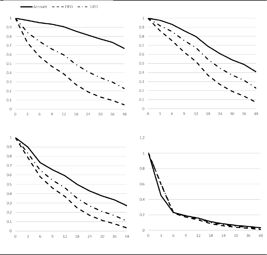
38
Figure 8: Evolution of the Remainder of Month 0 Balance at the Portfolio Level and Across Segments
(as a % of Initial Balance)
Figure 8.a: Low-risk segment
Figure 8.b: High-risk segment
Figure 8.c: Low-delinquency segment
Figure 8.d: High-delinquency segment
Note: The figures follow the evolution from month 0 of balances across segments of the portfolio as a percentage of initial
balances at the account level and at the loan level for specific payment allocation rules. These figures are consistent across
cohorts so we report only the aggregated evolution of balances across cohorts.

39
Figure 9: Portfolio Loss Curves Across Cohorts
Figure 9.a: Account loss curves
Figure 9.b: FIFO loss curves
Figure 9.c: (LIFO loss – FIFO loss)
Figure 9.d: LIFO loss curves
Note: 08Q1, 09Q1, 10Q1, etc. represent, respectively, cohorts with reference month as March of 2008, 2009, 2010, etc.

40
Figure 10: Portfolio Loss Curves Across Segments Low-Risk and High-Risk Revolver, High
Delinquent
Note: The figure depicts loss curves for the delinquent, high-risk and low-risk revolver segments. Curves are rank ordered
by risk so there is no need to differentiate across curves with additional notation.

41
Figure 11: Portfolio Loss Curves Across Cohorts and FIFO/LIFO Coverage Ratio
Note: The figure depicts loss curves across cohorts for different time spells (15, 18, etc.) in months. Loss curves
ordered, with longer spells are associated with higher loss severities. FIFO and LIFO loss curves are computed for the
life of the loan. The intersection of portfolio/segment loss curves with FIFO/LIFO loss curves provides a measure of the
coverage ratio for different cohort years (i.e., a measure of how many future months of actual portfolio loss are covered
by the corresponding allowance).

42
Figure 12: Loss Curves Across Cohorts and FIFO/LIFO Coverage Ratio
Figure 12.a: Revolver, low-risk segment
Figure 12.b: Revolver, high-risk segment
Figure 12.c: Low-delinquency segment
Figure 12.d: High-delinquency segment
Note: The figure depicts loss curves across cohorts for different time spells (15, 18, etc.) in months. Loss curves
ordered, with longer spells are associated with higher loss severities. FIFO and LIFO loss curves are computed for the
life of the loan or up to 5 years forward. The intersection of portfolio/segment loss curves with FIFO/LIFO loss curves
provides a measure of the coverage ratio for different cohort years.
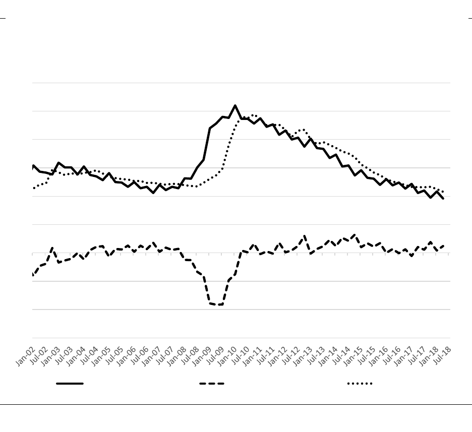
43
Figure 13: Unemployment Rate and Forecasting Error (4 quarters ahead)
Note: The figure depicts realized unemployment rate, 4 quarters ahead unemployment rate forecast and forecasting
error.
-6
-4
-2
0
2
4
6
8
10
12
Unemployment Rate and Forecasting Error (4 Q.
Ahead)
Unemployment Rate (UR) forecasting error 4Q ahead UR Forecast

44
Figure 14: FIFO Loss Projection Fit Over Time Over Macroeconomic Forecast Assumptions
Note: The figure depicts realized FIFO losses and model projected FIFO losses under two different macroeconomic
forecasts, perfect forecast, and 4 quarters ahead forecast (subject to forecasting error).
0
0.01
0.02
0.03
0.04
0.05
0.06
0.07
0.08
0.09
0.1
0.11
0.12
0.13
0.14
0.15
0.16
0.17
0.18
0.19
0.2
Fifo Projections Fit
FIFO realized Perfect Macro foresight Forecasterd Macro

45
Figure 15: Proportional Impact of Macroeconomic Forecasting Error
Note: The figure depicts forecasting error from using contemporaneous macroeconomic forecast and taking the model forecast
with perfect foresight as the “ideal” baseline. The graph depicts results separately for segments for low-risk, medium-risk, and
high-risk revolver accounts and for delinquent (30+ days past due) and seriously delinquent (60+ days past due) accounts.
-0.1
-0.05
0
0.05
0.1
0.15
0.2
0.25
0.3
0.35
0.4
0.45
Impact of Macro Forecasting Error (Proportional)
Low Risk Rev. Medium Risk Rev. High Risk Rev.
Low Risk Del. High Risk Del.

46
VII. References
Agarwal, S., and C. Liu (2003). “Determinants of Credit Card Delinquency and Bankruptcy:
Macroeconomic Factors,” Journal of Economics and Finance 27 (1), 75–85.
Banerjee, P., and J. Canals-Cerdá. “Credit Risk Analysis of Credit Card Portfolios Under Economic
Stress Conditions,” Banking and Finance Review 5:2 (December 2013).
Board of Governors of the Federal Reserve System. “Dodd–Frank Act Stress Test 2018: Supervisory
Stress Test Methodology and Results,” June 2018,
www.federalreserve.gov/publications/files/2018-dfast-methodology-results-20180621.pdf
.
Board of Governors of the Federal Reserve System, Federal Deposit Insurance Corporation, National
Credit Union Administration, Office of the Comptroller of the Currency. “Joint Statement on the New
Accounting Standard on Financial Instruments — Credit Losses,” June 17, 2016.
Board of Governors of the Federal Reserve System. “Frequently Asked Questions on the New
Accounting Standard on Financial Instruments — Credit Losses,”
www.federalreserve.gov/supervisionreg/topics/faq-new-accounting-standards-on-financial-
instruments-credit-losses.htm.
Board of Governors of the Federal Reserve System. “Regulatory Capital Rules: Implementation and
Transition of the Current Expected Credit Losses Methodology for Allowances and Related
Adjustments to the Regulatory Capital Rules and Conforming Amendments to Other Regulations,”
proposed rule by the Comptroller of the Currency, the Federal Reserve System, and the Federal
Deposit Insurance Corporation, May 14,
2018,
www.federalregister.gov/documents/2018/05/14/2018-08999/regulatory-capital-rules-
implementation-and-transition-of-the-current-expected-credit-losses.
Chae, Sarah, Robert F. Sarama, Cindy M. Vojtech, and James Wang (2018). “The Impact
of the Current Expected Credit Loss Standard (CECL) on the Timing and Comparability
of Reserves,” Finance and Economics Discussion Series 2018-020. Washington, D.C.: Board of
Governors of the Federal Reserve System, https://doi.org/10.17016/FEDS.2018.020
.

47
Canals-Cerdá, J. “Pro-Cyclicality of Capital and Portfolio Segmentation in the Advanced Internal
Ratings-Based Framework: An Application to Mortgage Portfolios,” Journal of Risk Model
Validation12:3 (September 2018), 1–27.
Canals-Cerdá, J., and S. Kerr. “Forecasting Credit Card Portfolio Losses in the Great Recession: A
Study in Model Risk,” Journal of Credit Risk 11:1 (March 2015), 29–57.
Covas, F., and W. Nelson (2018). “Current Expected Credit Loss: Lessons from 2007-2009,” Bank
Policy Institute, Staff Working Paper 2018-1.
DeRitis, C., and M. Zandi (2018). “Gauging CECL Cyclicality,” Moody’s Analytics, December 2018.
Financial Accounting Standards Board. “Accounting Standards Update 2016-13, Financial
Instruments — Credit Losses (Topic 326): Measurement of Credit Losses on Financial Instruments,”
June 2016.
Financial Accounting Standards Board, Transition Resource Group for Credit Losses. “Memo No. 5
Determining the Estimated Life of a Credit Card Receivable.” June 2017 TRG Meeting.
FR Y-14M Capital Assessment and Stress Testing, Domestic Credit Card Data Collection,
https://www.federalreserve.gov/apps/reportforms/reportdetail.aspx?sOoYJ+5BzDYnbIw+U9pka3
sMtCMopzoV.
Kalbfleisch, J. D., and R. L. Prentice. 2002. The Statistical Analysis of Failure Time Data. 2nd ed. New
York: Wiley.
Kaplan, E. L., and P. Meier. 1958. “Nonparametric Estimation from Incomplete Observations.”
Journal of the American Statistical Association 53: 457–481.
Li, Phillip, Qi, Min, Xiaofei Zhang and Xinlei Zhao. 2016. “Further Investigation of Parametric Loss
Given Default Modeling,” Journal of Credit Risk 12(4), 17–47.
48
Loudis, Bert, and Ben Ranish (2019). “CECL and the Credit Cycle,” Finance and Economics
Discussion Series 2019-061. Washington, D.C.: Board of Governors of the Federal Reserve System,
https://doi.org/10.17016/FEDS.2019.061.
