
CFA - practice
Confirmatory Factor Analysis in R

Intro
Today’s goal:
Teach how to do Confirmatory Factor Analysis in R.
Outline:
-
Example

CFA
Confirmatory Factor Analysis

Example
twq.dat, variables:
-
cgraph: inspectability (0: list, 1: graph)
-
citem-cfriend: control (baseline: no control)
-
cig (citem * cgraph) and cfg (cfriend * cgraph)
-
s1-s7: satisfaction with the system
-
q1-q6: perceived recommendation quality
-
c1-c5: perceived control
-
u1-u5: understandability

Example
twq.dat, variables:
-
e1-e4: user music expertise
-
t1-t6: propensity to trust
-
f1-f6: familiarity with recommenders
-
average rating of, and number of known items in, the top
10
-
time taken to inspect the recommendations

F1 F2
D E FA B C
.84 .91 .85 .89 .78 .92
.45
.29 .17 .28 .21 .39 .15
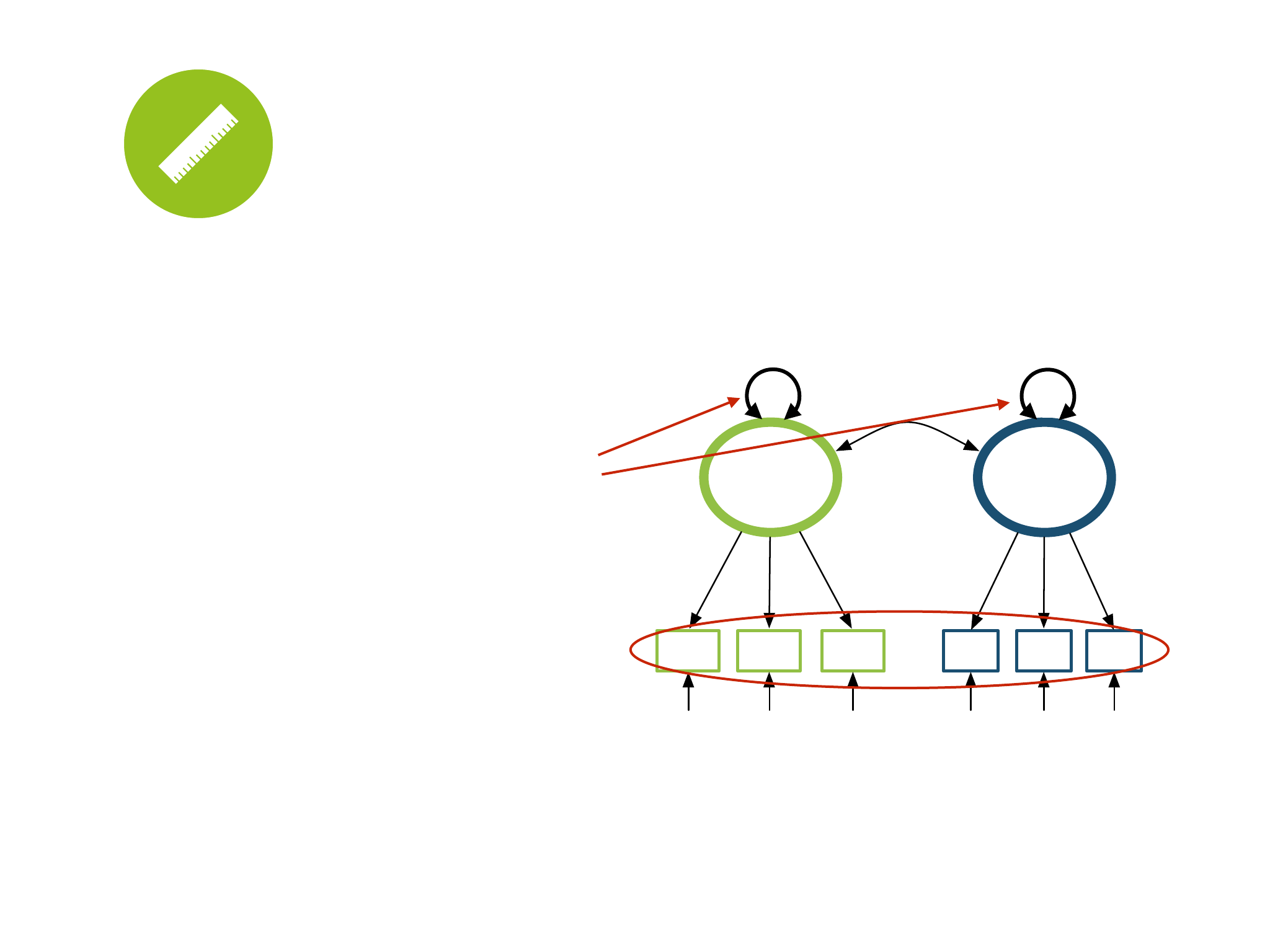
CFA syntax
model <- ‘
F1 =~ A+B+C
F2 =~ D+E+F
‘

F1 F2
D E FA B C
.84 .91 .85 .89 .78 .92
.45
.29 .17 .28 .21 .39 .15
CFA syntax
model <- ‘
F1 =~ A+B+C+E
F2 =~ D+E+F
‘
.50
.14

F1 F2
D E FA B C
.84 .91 .85 .89 .78 .92
.45
.29 .17 .28 .21 .39 .15
CFA syntax
model <- ‘
F1 =~ A+B+C
F2 =~ D+E+F
A ~~ E
‘
.50

F1 F2
D E FA B C
.84 .91 .85 .89 .78 .92
.45
.29 .17 .28 .21 .39 .15
CFA estimation
fit <- cfa(model, data=d)
1
1
assumed normally distributed ratio variables!
Unit Loading Identification (ULI)!

F1 F2
D E FA B C
.84 .91 .85 .89 .78 .92
.45
.29 .17 .28 .21 .39 .15
CFA estimation
fit <- cfa(model, data=d,
ordered = c(“A”, “B”, “C”,
“D”, “E”, “F”))
1
1
assumed ordered categorical!
F1 F2
D E FA B C
.84 .91 .85 .89 .78 .92
.45
.29 .17 .28 .21 .39 .15
CFA estimation
fit <- cfa(model, data=d,
ordered = c(“A”, “B”, “C”,
“D”, “E”, “F”), std.lv=T)
Unit Variance Identification (UVI)!
1 1
assumed ordered categorical!

CFA output
summary(fit, rsquare=T, fit.measures=T)
“rsquare” gives us 1-uniqueness values
“fit.measures” gives us CFI, TLI, and RMSEA

Run the CFA
Write model definition:
model <- ‘satisf =~ s1+s2+s3+s4+s5+s6+s7
quality =~ q1+q2+q3+q4+q5+q6
control =~ c1+c2+c3+c4+c5
underst =~ u1+u2+u3+u4+u5’
Run cfa (load package lavaan):
fit <- cfa(model, data=twq, ordered=names(twq), std.lv=TRUE)
Inspect model output:
summary(fit, rsquare=TRUE, fit.measures=TRUE)

Run the CFA
Output (model fit):
lavaan (0.5-17) converged normally after 39 iterations
Number of observations 267
Estimator DWLS Robust
Minimum Function Test Statistic 251.716 365.719
Degrees of freedom 224 224
P-value (Chi-square) 0.098 0.000
Scaling correction factor 1.012
Shift parameter 117.109
for simple second-order correction (Mplus variant)
Model test baseline model:
Minimum Function Test Statistic 48940.029 14801.250
Degrees of freedom 253 253
P-value 0.000 0.000
Note: we do not really care about this yet
(we should optimize our model first)

Run the CFA
Output (model fit, continued):
User model versus baseline model:
Comparative Fit Index (CFI) 0.999 0.990
Tucker-Lewis Index (TLI) 0.999 0.989
Root Mean Square Error of Approximation:
RMSEA 0.022 0.049
90 Percent Confidence Interval 0.000 0.034 0.040 0.058
P-value RMSEA <= 0.05 1.000 0.579
Weighted Root Mean Square Residual:
WRMR 0.855 0.855
Parameter estimates:
Information Expected
Standard Errors Robust.sem

Run the CFA
Output (loadings):
Estimate Std.err Z-value P(>|z|)
Latent variables:
satisf =~
s1 0.888 0.018 49.590 0.000
s2 -0.885 0.018 -48.737 0.000
s3 0.771 0.029 26.954 0.000
s4 0.821 0.025 32.363 0.000
s5 0.889 0.018 50.566 0.000
s6 0.788 0.031 25.358 0.000
s7 -0.845 0.022 -38.245 0.000
quality =~
q1 0.950 0.013 72.421 0.000
q2 0.949 0.013 72.948 0.000
q3 0.942 0.012 77.547 0.000
q4 0.805 0.033 24.257 0.000
q5 -0.699 0.042 -16.684 0.000
q6 -0.774 0.040 -19.373 0.000
These are the loadings (the regression bs on the arrows going from the factor to the item)
They should be > 0.70 (because R
2
= loading
2
should be > 0.5)
Negative loadings are for negative items (please check!!)

Run the CFA
Output (loadings, continued):
control =~
c1 0.712 0.038 18.684 0.000
c2 0.855 0.024 35.624 0.000
c3 0.905 0.022 41.698 0.000
c4 0.723 0.037 19.314 0.000
c5 -0.424 0.056 -7.571 0.000
underst =~
u1 -0.557 0.047 -11.785 0.000
u2 0.899 0.016 57.857 0.000
u3 0.737 0.030 24.753 0.000
u4 -0.918 0.016 -58.229 0.000
u5 0.984 0.010 97.787 0.000

Run the CFA
Output (factor correlations):
Covariances:
satisf ~~
quality 0.686 0.033 20.503 0.000
control -0.760 0.028 -26.913 0.000
underst 0.353 0.048 7.320 0.000
quality ~~
control -0.648 0.040 -16.041 0.000
underst 0.278 0.058 4.752 0.000
control ~~
underst -0.382 0.051 -7.486 0.000
These are the factor correlations (the numbers on the arrows going from one factor to another)
They should not be too high (more about this later)
Note: the control factor turns out to be “lack of control” (that happens sometimes)

Run the CFA
Output (thresholds):
Thresholds:
s1|t1 -1.829 0.148 -12.382 0.000
s1|t2 -1.021 0.093 -10.941 0.000
s1|t3 -0.441 0.080 -5.539 0.000
s1|t4 0.874 0.089 9.874 0.000
s2|t1 -0.330 0.078 -4.207 0.000
s2|t2 0.732 0.085 8.626 0.000
s2|t3 1.157 0.099 11.712 0.000
s2|t4 2.005 0.170 11.790 0.000
s3|t1 -1.737 0.138 -12.581 0.000
s3|t2 -0.834 0.087 -9.540 0.000
s3|t3 -0.222 0.078 -2.869 0.004
s3|t4 1.176 0.100 11.800 0.000
s4|t1 -1.696 0.134 -12.642 0.000
s4|t2 -0.732 0.085 -8.626 0.000
s4|t3 -0.014 0.077 -0.183 0.855
s4|t4 1.037 0.094 11.043 0.000
s5|t1 -1.622 0.128 -12.710 0.000
s5|t2 -0.769 0.086 -8.972 0.000
s5|t3 -0.118 0.077 -1.527 0.127
s5|t4 1.087 0.096 11.339 0.000
s6|t1 -1.737 0.138 -12.581 0.000
s6|t2 -0.902 0.089 -10.094 0.000
s6|t3 0.441 0.080 5.539 0.000
... ... ... ... ...
These are the thresholds for the ordered categorical variables
P(Y)
0
0.2
0.4
0.6
0.8
1
U
-7
-6
-5
-4
-3
-2
-1
0
1
2
3
4
5
6
we predict 1 2
3 4 5

Run the CFA
Output (variances):
Variances:
s1 0.212
s2 0.218
s3 0.406
s4 0.326
s5 0.210
s6 0.379
s7 0.286
q1 0.097
q2 0.099
q3 0.112
q4 0.352
q5 0.511
q6 0.401
c1 0.494
c2 0.269
c3 0.180
c4 0.478
c5 0.821
u1 0.690
u2 0.192
u3 0.456
u4 0.157
u5 0.032
satisf 1.000
quality 1.000
control 1.000
underst 1.000
The variances of the items (observed)
The variances of the factors (fixed to 1, using UVI)

Run the CFA
Output (r-square):
R-Square:
s1 0.788
s2 0.782
s3 0.594
s4 0.674
s5 0.790
s6 0.621
s7 0.714
q1 0.903
q2 0.901
q3 0.888
q4 0.648
q5 0.489
q6 0.599
c1 0.506
c2 0.731
c3 0.820
c4 0.522
c5 0.179
u1 0.310
u2 0.808
u3 0.544
u4 0.843
u5 0.968
Also called “variance extracted” or “communality”… it is 1 – uniqueness
Should be > 0.50 (or at the very least > 0.40)

Improve the model
Remove items with low communality
check for r-square < 0.40 (or maybe 0.50)
Remove items with high cross-loadings or residual
correlations
check the modification indices
Keep at least three items
if necessary, specify a model with cross-loadings or residual
correlations… but try to avoid this!

Low communality
Based on r-square, iteratively remove items:
c5 (r-squared = 0.180)
u1 (r-squared = 0.324)

High residuals
High residual correlations:
-
The observed correlation between two items is
significantly higher (or lower) than predicted
-
Might mean that factors should be split up
High cross-loadings:
-
When the model suggest that the model fits significantly
better if an item also loads on an additional factor
-
Could mean that an item actually measures two things

High residuals
In R: modification indices
Modification indices give an estimate on how each possible
adjustment of the model may improve it
Listed are:
mi: the modification index (a chi-square value with 1 df)
epc: the expected value of the parameter if added to the
model

High residuals
Get the modification indices
mods <- modindices(fit, power=TRUE)
Only keep the ones that are significant and large enough to
be interesting
mods <- mods[grep("\\*", mods$decision),]
Display
mods

High residuals
Look for items involved in several modifications that have a
high mi (most important), high epc (less important), or both
Remove the most troublesome one from the model
In this case: u3
Loads on satisfaction and quality, correlates with c1 and s6
Recalculate the modification indices
(etc.)

Improve the model
For all these metrics:
-
Remove items that do not meet the criteria, but be careful
to keep at least 3 items per factor
-
One may remove an item that has values much worse
than other items, even if it meets the criteria
(Because of this, I’m going to stop here)
(note: there could be something going on with satisfaction;
let’s explore later…)

Inspect the model
Inspect the following things in the final model:
Item-fit (this should be good by now)
Factor-fit: Average Variance Extracted
Model-fit: Chi-square test, CFI, TLI, RMSEA

Item-fit
Output (loadings):
Latent variables:
satisf =~
s1 0.888 0.018 50.049 0.000
s2 -0.885 0.018 -49.187 0.000
s3 0.769 0.029 26.847 0.000
s4 0.822 0.025 32.660 0.000
s5 0.889 0.017 51.012 0.000
s6 0.786 0.031 25.139 0.000
s7 -0.845 0.022 -38.547 0.000
quality =~
q1 0.950 0.013 72.301 0.000
q2 0.950 0.013 73.136 0.000
q3 0.942 0.012 77.787 0.000
q4 0.804 0.033 24.346 0.000
q5 -0.698 0.042 -16.693 0.000
q6 -0.775 0.040 -19.510 0.000
control =~
c1 0.700 0.039 17.958 0.000
c2 0.859 0.024 36.386 0.000
c3 0.911 0.022 41.986 0.000
c4 0.717 0.038 18.773 0.000
underst =~
u2 0.910 0.014 63.720 0.000
u4 -0.922 0.016 -58.796 0.000
u5 0.984 0.010 93.772 0.000
All remaining loadings > 0.70

Item-fit
Output (factor correlations):
Covariances:
satisf ~~
quality 0.687 0.033 20.507 0.000
control -0.762 0.029 -26.711 0.000
underst 0.315 0.052 6.105 0.000
quality ~~
control -0.646 0.041 -15.718 0.000
underst 0.263 0.059 4.494 0.000
control ~~
underst -0.328 0.058 -5.681 0.000

Item-fit
Output (r-square):
R-Square:
s1 0.788
s2 0.783
s3 0.592
s4 0.675
s5 0.791
s6 0.617
s7 0.714
q1 0.902
q2 0.902
q3 0.887
q4 0.646
q5 0.487
q6 0.601
c1 0.490
c2 0.738
c3 0.830
c4 0.514
u2 0.828
u4 0.849
u5 0.968
A few are < 0.50, but all are > 0.48, so this is quite okay

Factor-fit
Average Variance Extracted (AVE)
In lavaan output: average of R-squared per factor
Convergent validity:
AVE > 0.5
Discriminant validity
√(AVE) > largest correlation with other factors

Factor-fit
Satisfaction:
AVE = 0.709, √(AVE) = 0.842, largest correlation = 0.762
Quality:
AVE = 0.737, √(AVE) = 0.859, largest correlation = 0.687
Control:
AVE = 0.643, √(AVE) = 0.802, largest correlation = 0.762
Understandability:
AVE = 0.874, √(AVE) = 0.935, largest correlation = 0.341

Model-fit metrics
Chi-square test of model fit:
-
Tests whether there any significant misfit between
estimated and observed correlation matrix
-
Often this is true (p < .05)… models are rarely perfect!
-
Alternative metric: chi-squared / df < 3 (good fit) or < 2
(great fit)

Model-fit metrics
CFI and TLI:
-
Relative improvement over baseline model; ranging from
0.00 to 1.00
-
CFI should be > 0.96 and TLI should be > 0.95
RMSEA:
-
Root mean square error of approximation
-
Overall measure of misfit
-
Should be < 0.05, and its confidence interval should not
exceed 0.10.

Model-fit metrics
Output (model fit):
lavaan (0.5-17) converged normally after 38 iterations
Number of observations 267
Estimator DWLS Robust
Minimum Function Test Statistic 162.211 286.057
Degrees of freedom 164 164
P-value (Chi-square) 0.525 0.000
Scaling correction factor 0.755
Shift parameter 71.330
for simple second-order correction (Mplus variant)
Model test baseline model:
Minimum Function Test Statistic 46290.833 14383.462
Degrees of freedom 190 190
P-value 0.000 0.000
Model shows significant misfit, but
Chi-square / df is good:
286 / 164 = 1.76
This tests if the model is better
than the worst possible model
(unsurprisingly, it is…)

Run the CFA
Output (model fit, continued):
User model versus baseline model:
Comparative Fit Index (CFI) 1.000 0.991
Tucker-Lewis Index (TLI) 1.000 0.990
Root Mean Square Error of Approximation:
RMSEA 0.000 0.053
90 Percent Confidence Interval 0.000 0.027 0.043 0.063
P-value RMSEA <= 0.05 1.000 0.311
Weighted Root Mean Square Residual:
WRMR 0.777 0.777
Parameter estimates:
Information Expected
Standard Errors Robust.sem
CFI and TLI are excellent
RMSEA = .053 is not great, but the 90%
CI is ok: [.043, .063] (not > .10)
You can ignore WRMR

Summary
Specify and run your CFA
Alter the model until all remaining items fit
Make sure you have at least 3 items per factor!
Report final loadings, factor fit, and model fit

Summary
We conducted a CFA and examined the validity and
reliability scores of the constructs measured in our study.
Upon inspection of the CFA model, we removed items c5
(communality: 0.180) and u1 (communality: 0.324), as well as
item u3 (high cross-loadings with several other factors). The
remaining items shared at least 48% of their variance with
their designated construct.

Summary
To ensure the convergent validity of constructs, we examined
the average variance extracted (AVE) of each construct.
The AVEs were all higher than the recommended value of
0.50, indicating adequate convergent validity.
To ensure discriminant validity, we ascertained that the
square root of the AVE for each construct was higher than
the correlations of the construct with other constructs.

Summary
Construct
Item
Loading
System
satisfaction
Alpha: 0.92
AVE: 0.709
I would recommend TasteWeights to others.
0.888
TasteWeights is useless.
-0.885
TasteWeights makes me more aware of my choice options.
0.768
I can make better music choices with TasteWeights.
0.822
I can find better music using TasteWeights.
0.889
Using TasteWeights is a pleasant experience.
0.786
TasteWeights has no real benefit for me.
-0.845
Perceived
Recommendation
Quality
Alpha: 0.90
AVE: 0.737
I liked the artists/bands recommended by the TasteWeights
system.
0.950
The recommended artists/bands fitted my preference.
0.950
The recommended artists/bands were well chosen.
0.942
The recommended artists/bands were relevant.
0.804
TasteWeights recommended too many bad artists/bands.
-0.697
I didn't like any of the recommended artists/bands.
-0.775
Perceived
Control
Alpha: 0.84
AVE: 0.643
I had limited control over the way TasteWeights made
recommendations.
0.700
TasteWeights restricted me in my choice of music.
0.859
Compared to how I normally get recommendations,
TasteWeights was very limited.
0.911
I would like to have more control over the recommendations.
0.716
I decided which information was used for recommendations.
Understandability
Alpha: 0.92
AVE: 0.874
The recommendation process is not transparent.
I understand how TasteWeights came up with the
recommendations.
0.893
TasteWeights explained the reasoning behind the
recommendations.
I am unsure how the recommendations were generated.
-0.923
The recommendation process is clear to me.
0.987
Construct
Item
Loading
Response Frequencies
-2
-1
0
1
2
System
satisfaction
Alpha: 0.92
AVE: 0.709
I would recommend TasteWeights to others.
0.888
9
32
47
128
51
TasteWeights is useless. -0.885 99 106 29 27 6
TasteWeights makes me more aware of my choice options. 0.768 11 43 56 125 32
I can make better music choices with TasteWeights. 0.822 12 50 70 95 40
I can find better music using TasteWeights. 0.889 14 45 62 109 37
Using TasteWeights is a pleasant experience. 0.786 0 11 38 130 88
TasteWeights has no real benefit for me. -0.845 56 91 49 53 18
Perceived
Recommendation
Quality
Alpha: 0.90
AVE: 0.737
I liked the artists/bands recommended by the TasteWeights
system.
0.950 6 30 27 125 79
The recommended artists/bands fitted my preference. 0.950 10 30 24 123 80
The recommended artists/bands were well chosen. 0.942 10 35 26 101 95
The recommended artists/bands were relevant. 0.804 4 18 14 120 111
TasteWeights recommended too many bad artists/bands. -0.697 104 88 45 20 10
I didn't like any of the recommended artists/bands. -0.775 174 61 16 14 2
Perceived
Control
Alpha: 0.84
AVE: 0.643
I had limited control over the way TasteWeights made
recommendations.
0.700 13 52 48 112 42
TasteWeights restricted me in my choice of music. 0.859 40 90 45 76 16
Compared to how I normally get recommendations,
TasteWeights was very limited.
0.911 36 86 53 68 24
I would like to have more control over the recommendations. 0.716 8 27 38 130 64
I decided which information was used for recommendations. 42 82 50 79 14
Understandability
Alpha: 0.92
AVE: 0.874
The recommendation process is not transparent. 24 77 76 68 22
I understand how TasteWeights came up with the
recommendations.
0.893 8 41 17 127 74
TasteWeights explained the reasoning behind the
recommendations.
28 59 46 91 43
I am unsure how the recommendations were generated. -0.923 71 90 28 62 16
The recommendation process is clear to me. 0.987 14 65 23 101 64

Summary
Alpha
AVE
Satisfaction
Quality
Control
Underst.
Satisfaction
0.92
0.709
0.842
0.687
–0.762
0.336
Quality
0.90
0.737
0.687
0.859
–0.646
0.282
Control
0.84
0.643
–0.762
–0.646
0.802
–0.341
Underst.
0.92
0.874
0.336
0.282
–0.341
0.935
diagonal: √(AVE)
off-diagonal: correlations

Alternative models
s3 and s4 are more highly correlated, so:
emodel <- ‘satisf =~ s1+s2+s5+s6+s7
choice =~ s3+s4
quality =~ q1+q2+q3+q4+q5+q6
control =~ c1+c2+c3+c4+c5
underst =~ u1+u2+u3+u4+u5’
Run cfa:
efit <- cfa(emodel, data=twq, ordered=names(twq), std.lv=T)
Inspect model output:
summary(efit, rsquare=TRUE, fit.measures=TRUE)

Factor-fit
Satisfaction: AVE = 0.744, √(AVE) = 0.863
Choice satisfaction: AVE = 0.782, √(AVE) = 0.884
Correlation between them = 0.889
Conclusion: no discriminant validity!

Alternative models
s3 and s4 are more highly correlated, so:
fmodel <- ‘satisf =~ s1+s2+s3+s4+s5+s6+s7
quality =~ q1+q2+q3+q4+q5+q6
control =~ c1+c2+c3+c4+c5
underst =~ u1+u2+u3+u4+u5
s3 ~~ s4’
Run cfa and inspect output:
ffit <- cfa(emodel, data=twq, ordered=names(twq), std.lv=T)
summary(ffit, rsquare=TRUE, fit.measures=TRUE)

“It is the mark of a truly intelligent person !
to be moved by statistics.”
George Bernard Shaw!
