
FEDERAL RESERVE BANK OF SAN FRANCISCO
WORKING PAPER SERIES
The Long-Run Effects of Monetary Policy
Òscar Jordà
Federal Reserve Bank of San Francisco
University of California, Davis
Sanjay R. Singh
Federal Reserve Bank of San Francisco
University of California, Davis
Alan M. Taylor
Columbia University
NBER and CEPR
May 2023
Working Paper 2020-01
https://www.frbsf.org/economic-research/publications/working-papers/2020/01/
Suggested citation:
Jordà, Òscar, Sanjay R. Singh, Alan M. Taylor. 2023. “The long-run effects of monetary
policy
,” Federal Reserve Bank of San Francisco Working Paper 2020-01.
https://doi.org/10.24148/wp2020-01
The views in this paper are solely the responsibility of the authors and should not be interpreted
as reflecting the views of the Federal Reserve Bank of San Francisco or the Board of Governors
of the Federal Reserve System.

The long-run effects of monetary policy
⋆
`
Oscar Jord`a
†
Sanjay R. Singh
§
Alan M. Taylor
‡
May 2023
Abstract
We document that the real effects of monetary shocks last for over a decade. Our approach
relies on (1) identification of exogenous and non-systematic monetary shocks using the
trilemma of international finance; (2) merged data from two new international historical
cross-country databases; and (3) econometric methods robust to long-horizon inconsistent
estimates. Notably, the capital stock and total factor productivity (TFP) exhibit greater
hysteresis than labor. When we allow for asymmetry, we find these effects with tightening
shocks, but not with loosening shocks. When extending the horizon of the responses
reported in several recent studies that use alternative monetary shocks, we find similarly
persistent real effects, thus supporting our main findings.
JEL classification codes: E01, E30, E32, E44, E47, E51, F33, F42, F44.
Keywords: monetary policy, money neutrality, hysteresis, trilemma, instrumental variables,
local projections.
⋆
We are thankful to Sushant Acharya, George-Marios Angeletos, Gadi Barlevy, Susanto Basu, Saki Bigio,
Edouard Challe, Lawrence Christiano, James Cloyne, Julian di Giovanni, St´ephane Dupraz, Martin Eichenbaum,
Charles Engel, Gauti Eggertsson, Antonio Fat´as, John Fernald, Luca Fornaro, Jordi Gal´ı, Georgios Georgiadis,
Yuriy Gorodnichenko, Pierre-Olivier Gourinchas, James Hamilton, Oleg Itskhoki, Jean-Paul L’Huillier, Silvia
Miranda-Agrippino, Dmitry Mukhin, Juan Pablo Nicolini, Pascal Paul, Albert Queralto, Valerie Ramey, Ina
Simonovska, J´on Steinsson, Andrea Tambalotti, Silvana Tenreyro, Mart´ın Uribe, Johannes Wieland, who
provided very helpful comments and suggestions, as did many seminar and conference participants at the
Barcelona Summer Forum, the NBER Summer Institute IFM and EFCE Program Meetings, the Econometric
Society World Congress, the SED Annual Meeting, the ASSA Meetings, Bank of England, the Federal Reserve
Banks of Richmond, San Francisco, St. Louis, and Board of Governors, CEPR MEF Seminar Series, the Midwest
Macro Conference, Northwestern University, Delhi School of Economics, ISI Delhi, IGIDR Mumbai, Salento
Macro, Claremont McKenna College, the Swiss National Bank, the Bank of Spain, the Norges Bank, the Bank
of Finland, Danmarks Nationalbank, Columbia SIPA, UC Berkeley, UC Davis, UC Irvine, UCLA, UC San
Diego, University of Wisconsin–Madison, Universit¨at Z¨urich, Vanderbilt University, Asian School of Business,
and Trinity College, Dublin. Antonin Bergeaud graciously shared detailed data from the long-term productivity
database created with Gilbert Cette and R´emy Lecat at the Banque de France. All errors are ours. The views
expressed herein are solely those of the authors and do not necessarily represent the views of the Federal Reserve
Bank of San Francisco or the Federal Reserve System.
†
Federal Reserve Bank of San Francisco and Department of Economics, University of California, Davis
§
Federal Reserve Bank of San Francisco and Department of Economics, University of California, Davis
(sanjay[email protected]; [email protected]).
‡
Columbia University; NBER; and CEPR (amt2314@columbia.edu).

Are there circumstances in which changes in aggregate demand can have an appreciable,
persistent effect on aggregate supply?
— Yellen (2016)
1. Introduction
What is the effect of monetary policy on the long-run productive capacity of the economy?
Since at least Hume (1752), macroeconomics has largely operated under the assumption that
money is neutral in the long-run, and a vast literature spanning centuries has gradually built
the case (see, for example, King and Watson, 1997, for a review). Contrary to this monetary
canon, we find evidence rejecting long-run neutrality.
Our investigation of monetary neutrality rests on three pillars. First, it is essential to
identify exogenous movements in interest rates to obtain a reliable measure of monetary effects
and avoid confounding. Second, because we focus on long-run outcomes, we rely on a panel
of countries observed over as long a period as we can to maximize data span and, hence, the
statistical power of our conclusions. Third, as we show below, the empirical method used can
make a big difference: common approaches are designed to maximize short-horizon fit, but we
need methods that are consistent over longer spans of time. We discuss how we build on each
of these three pillars next.
On identification, the first pillar, in section 2 we exploit the trilemma of international finance
(see, for example, Obstfeld, Shambaugh, and Taylor, 2004, 2005; Shambaugh, 2004). The
key idea is that when a country pegs its currency to some base currency with free movement
of capital across borders, it loses control—at least to some degree—over its interest rate: a
correlation in home and base interest rates is thus induced, which is exact when the peg is
hard and arbitrage frictionless, but is generally less than one otherwise. Insofar as base rates
are determined by base country conditions alone, they provide a potential source of exogenous
variation in home rates. We theoretically ground this identification strategy in a canonical New
Keynesian small open economy model (Schmitt-Groh´e and Uribe, 2016; Fornaro and Romei,
2019; Bianchi and Lorenzoni, 2022). Specifically, we derive analytical results to show formally,
for the first time, how a trilemma-based identification approach recovers the monetary policy
impulse response function of interest. Moreover, we exploit the model to provide bounds on
failures of the exclusion restriction due to spillover effects.
1
Second, moving on to the data pillar, in section 3 we rely on two recent macro-history
databases spanning 125 years and 17 advanced economies. First, we use the data in Jord`a,
1
We leverage the insights of open-economy literature to show how theory maps rigorously into our trilemma
identification scheme and guides an econometric approach that builds on earlier work in this vein (di Giovanni,
McCrary, and Von Wachter, 2009; Jord`a, Schularick, and Taylor, 2020).
1

Schularick, and Taylor (2017), available at
www.macrohistory.net/database
. This “JST
Database” contains key macroeconomic series, such as output, interest rates, as well as inflation,
credit, and many other potentially useful control variables for our analysis. Second, to allow
for a Solow decomposition of output into its components, we merge and incorporate data from
Bergeaud, Cette, and Lecat (2016), available at
http://www.longtermproductivity.com
.
2
Their data series include observations on investment in machines and buildings, number of
employees, and hours worked. With these variables, we construct measures of total factor
productivity (TFP), including with utilization adjustment, and then decompose impulse
responses for output into TFP, capital input, and labor input, to explore the channels of the
hysteresis that we have uncovered.
The third and final pillar of our analysis in section 4 has to do with the econometric approach.
We use local projections (Jord`a, 2005) in order to get more accurate estimates of the impulse
response function (IRF) at longer horizons. As we show formally, as long as the truncation
lag in local projections is chosen to grow with the sample size (at a particular rate that we
make specific below), local projections (LPs) estimate the impulse response consistently at any
horizon. In fact, as recently shown by Xu (2023), local projections are semi-parametrically
efficient in settings were the lag order may be infinite and the truncation lag is allowed to grow
with the sample. Other procedures commonly used to estimate impulse responses do not have
this property (see, for example, Lewis and Reinsel, 1985; Kuersteiner, 2005), and this—among
several other reasons—may explain the failure of some of the prior literature to discern the
highly persistent effects that we document here. See also, Plagborg-Møller and Wolf (2021);
Li, Plagborg-Møller, and Wolf (2022) for related results on comparison of LPs with vector
autoregressions (VARs).
Supported by these three pillars in section 5 we show that, surprisingly, monetary policy
affects the productive capacity of the economy for a very long time. In response to an exogenous
monetary shock, output declines and does not return to its pre-shock trend even twelve years
thereafter. Next, we investigate the source of this hysteresis and find that capital and TFP
experience similar trajectories to output. In contrast, total hours worked (both hours per
worker and number of workers) return more quickly to the original trend. Hence, our new
findings are distinct from the usual labor hysteresis mechanism previously emphasized in the
literature (see, for example, Blanchard and Summers, 1986; Gal´ı, 2015a; Blanchard, 2018; Gal´ı,
2020).
After a series of robustness checks, in section 6 we show that the responses display a key
asymmetry, or nonlinearity, with hysteresis forces much stronger after tightening shocks than
2
We are particularly thankful to Antonin Bergeaud for sharing some of the disaggregated series from their
database that we use to construct our own series of adjusted TFP.
2

loosening shocks, consistent with prior research on shorter-horizon response asymmetries (for
example, Tenreyro and Thwaites, 2016; Angrist, Jord`a, and Kuersteiner, 2018). Tight monetary
policy has long lasting effects, but loose monetary policy does not stimulate growth. The
asymmetries that we find echo results from models with downward nominal wage rigidity
(DNWR), though other mechanisms are possible.
3
How do our findings stack up against the state of knowledge? A voluminous literature
based on post-WW2 U.S. data has examined the causal effects of monetary policy (see, for
example, Christiano, Eichenbaum, and Evans, 1999; Ramey, 2016; Nakamura and Steinsson,
2018, provide a detailed review), but the evidence on long-run neutrality is, at best, mixed
(King and Watson, 1997). An important exception is the work of Bernanke and Mihov (1998),
which fails to reject long-run neutrality, but finds that the point estimates of GDP response to
monetary innovations do not revert to zero even after ten years. Mankiw (2001) interprets this
non-reversal as potential evidence of long-run non-neutrality.
4
In section 7, we relate our work to recent studies that employ different methods to identify
monetary shocks for the U.S. and the U.K. economies. Using their replication codes, we extend
the original estimates from published studies to eight-year horizons and, in fact, find similar
evidence of long-run non-neutral effects of monetary shocks. Miranda-Agrippino and Ricco
(2021) estimate a Bayesian VAR(12) for the U.S. economy with high-frequency market-based
monetary surprises around Federal Open Market Committee announcements (G¨urkaynak,
Sack, and Swanson, 2005) and Federal Reserve’s Greenbook forecasts. Brunnermeier, Palia,
Sastry, and Sims (2021) estimate a large-scale Bayesian SVAR model, for the U.S. economy,
with identification based on heteroskedasticity. Cesa-Bianchi, Thwaites, and Vicondoa (2020)
estimate a proxy structural VAR, for the U.K. economy, with their constructed high-frequency
monetary surprises measured around monetary policy announcements of the Bank of England.
Finally, our paper has been followed by a more recent literature that examines long-run
effects of transitory shocks. Antolin-Diaz and Surico (2022) document persistent effects of
transitory government spending shocks. Cloyne, Mart´ınez, Mumtaz, and Surico (2022) find
evidence for long-run effects of transitory corporate tax shocks. Furlanetto, Lepetit, Robstad,
Rubio-Ram´ırez, and Ulvedal (2021) also find that demand shocks have hysteresis effects for
3
On DNWR see, for example, Akerlof, Dickens, and Perry (1996), Benigno and Ricci (2011), Schmitt-Groh´e
and Uribe (2016), Barnichon, Debortoli, and Matthes (2021), Bianchi, Ottonello, and Presno (Forthcoming),
Born, D’Ascanio, M¨uller, and Pfeifer (2022).
4
Mankiw notes (emphasis added): “Bernanke and Mihov estimate a structural vector autoregression and
present the impulse response functions for real GDP in response to a monetary policy shock. (See their Figure
III.) Their estimated impulse response function does not die out toward zero, as is required by long-run neutrality.
Instead, the point estimates imply a large impact of monetary policy on GDP even after ten years. Bernanke
and Mihov don’t emphasize this fact because the standard errors rise with the time horizon. Thus, if we look
out far enough, the estimated impact becomes statistically insignificant. But if one does not approach the data
with a prior view favoring long- run neutrality, one would not leave the data with that posterior. The data’s best
guess is that monetary shocks leave permanent scars on the economy.” See also Gal´ı (1998).
3

the U.S. economy using a structural VAR model identified with short-run sign and long-run
zero restrictions. A theoretical literature at the intersection of endogenous productivity growth
and business cycles following the seminal work by Stadler (1990) provides micro-foundations
for hysteresis effects of transitory shocks. Cerra, Fat´as, and Saxena (2023) provide a recent
review of literature on hysteresis and business cycles. Complementary to our paper, theoretical
analyses by Benigno and Fornaro (2018) and Fornaro and Wolf (2022) link low nominal interest
rates to the rate of growth of productivity.
5
Going beyond our paper, hysteresis matters for
how we build models of monetary economies and what optimal monetary policy is in those
models: the welfare implications could be substantial (Benigno and Benigno, 2003; Benigno
and Woodford, 2012; Garga and Singh, 2021).
6
2. Identification via the trilemma
The trilemma of international finance gives a theoretically justified source of exogenous variation
in interest rates (Jord`a, Schularick, and Taylor, 2020). The logic is straightforward: under
a hard peg with perfect capital mobility, returns on similarly risky assets will be arbitraged
between the pegging (home) and pegged to (base) economies. In ideal frictionless settings,
strict interest parity would imply that rates are exactly correlated.
In reality this correlation is less than perfect, of course. But even under soft pegs (or dirty
floats), with frictions or imperfect arbitrage, a non-zero interest rate correlation between a home
economy and the base economy to which it pegs its exchange rate is enough for identification
using instrumental variables. In this section we present an open economy model to make formal
the conditions for identification, even in the presence of spillovers via non–interest rate channels
(or in the parlance of instrumental variables, violations of the exclusion restriction). This level
of detail allows us to construct econometric estimation procedures via propositions derived
from the model.
2.1. The identification problem in a nutshell
In measuring the effect of exogenous changes in domestic interest rates on output, consider
the simplest possible setup. For reasons that will become clear momentarily, we express all
variables in deviations from steady state (denoted with hats) so as to follow the same notation
5
See, among others, Fat´as (2000); Barlevy (2004); Anzoategui, Com´ın, Gertler, and Mart´ınez (2019); Bianchi,
Kung, and Morales (2019); Guerron-Quintana and Jinnai (2019); Queralto (2020); Schm¨oller and Spitzer (2021);
Vinci and Licandro (2021).
6
Our paper is also tangentially related to literature on productivity research. Baqaee and Farhi (2019)
construct a general framework where monetary shocks may affect allocative efficiency. Meier and Reinelt
(Forthcoming) provide evidence of increased misallocation following contractionary monetary policy shocks.
4

of the economic model that will follow. Hence, let
ˆ
Y
t
denote output;
ˆ
R
n
t
the home interest rate;
and
ˆ
R
∗
t
as base-country interest rates to which the home economy pegs its exchange rate. The
idea is to estimate β in the following regression:
ˆ
Y
t
=
ˆ
R
n
t
β + v
t
(1)
using
ˆ
R
∗
t
as an instrument (di Giovanni, McCrary, and Von Wachter, 2009; Jord`a, Schularick,
and Taylor, 2020). Base country interest rates seem likely to be determined by base country
economic conditions alone. Hence variation might be assumed to be essentially exogenous with
respect to the home economy considered.
However, does the exclusion restriction hold? What if, aside from the interest rates, there
are spillover channels from the base to the home country? That is, is there a direct channel by
which
ˆ
R
∗
t
affects
ˆ
Y
t
? If that is the case, then the regression really should be:
ˆ
Y
t
=
ˆ
R
n
t
β +
ˆ
R
∗
t
θ + u
t
(2)
It is easy to show that the IV estimator in Equation 1 would have a bias given by:
ˆ
β → β +
E(
ˆ
R
∗2
t
) θ
E(
ˆ
R
∗
t
ˆ
R
n
t
)
(3)
which will be non-zero as long as
θ ̸
= 0. However, if
θ
were known, then Equation 1 could be
estimated by instrumental variables by redefining the left-hand side as:
(
ˆ
Y
t
−
ˆ
R
∗
t
θ) =
ˆ
R
n
t
β + u
t
(4)
This observation was made, for example, by Conley, Hansen, and Rossi (2012).
In what follows, we derive an economic model that allows us to carefully work out the
exogeneity conditions of
ˆ
R
∗
t
and then determine the appropriate adjustments for potential
spillovers (the θ that results in the violation of the exclusion restriction).
2.2. Theory to guide identification
We build on a standard open economy setup widely used today as in Schmitt-Groh´e and Uribe
(2016), Fornaro and Romei (2019), and Bianchi and Lorenzoni (2022).
7
Our aim is not a new
model, but how theory maps rigorously into our trilemma identification scheme and guides our
econometric approach to identification. As the model is standard, many details are relegated
7
Elements of this framework appear in Benigno, Fornaro, and Wolf (2020), Farhi and Werning (2017), and
Fornaro (2015), among others. A textbook treatment is Schmitt-Groh´e, Uribe, and Woodford (2022, Ch. 13).
5

to the Appendix. In Appendix H, we obtain similar results in a Mundell-Fleming-Dornbusch
model with additional financial channels, as in Gourinchas (2018).
We assume that there is perfect foresight. The environment features incomplete international
markets with nominal rigidities. We focus on two countries: a large economy that we label the
base and a small open economy, the home country. We begin by describing a benchmark small
open economy. We want to recover the impulse response of output to a monetary shock in this
benchmark economy using trilemma identification.
2.3. Benchmark economy
Households. There is a continuum of measure one of identical households. Each household
receives an endowment of tradables
Y
T t
every period. The household preferences are given by
lifetime utility function
max
{C
t
,l
t
,B
t+1
}
E
0
∞
X
t=0
ζ
t
log(C
t
) − φ
l
1+ν
t
1 + ν
.
where
ζ
denotes the discount factor,
ν
is the (inverse) Frisch elasticity of labor supply,
φ
is a
scaling parameter to normalize
l
= 1 in the steady state, and
E
0
[·]
is the expectation operator
conditional on information available until date 0. The composite good
C
t
is a Cobb-Douglas
aggregate
C
t
=
C
T t
ω
ω
C
Nt
1−ω
1−ω
of a tradable good
C
T t
and a non-tradable good
C
Nt
, where
ω ∈ (0, 1) is the tradable share.
Households can trade in one-period riskless real and nominal bonds. Real bonds are
denominated in units of the tradable consumption good and pay gross interest rate
R
t
, taken
as given (i.e., a world real interest rate). Nominal bonds issued by the domestic central bank
are denominated in units of domestic currency, and pay gross nominal interest rate
R
n
t
. The
households’ budget constraint in units of domestic currency is then
P
T t
C
T t
+ P
Nt
C
Nt
+ P
T t
d
t
+ B
t
= W
t
l
t
+ P
T t
Y
T t
+ P
T t
d
t+1
R
t
+
B
t+1
R
n
t
+ T
t
+ Z
t
.
where
P
T t
and
P
Nt
are the prices of tradable and non-tradable goods in local currency;
d
t
is
the level of real debt in units of tradable good assumed in period
t −
1 and due in period
t
;
B
t
is the level of nominal debt in units of local currency assumed in period
t −
1 and due in period
t
;
W
t
is the nominal wage per unit of labor employed;
T
t
are nominal lump-sum transfers from
the government; and Z
t
nominal profits from domestic firms owned by households.
8
The household chooses a sequence of
{C
T t
, C
Nt
, l
t
, d
t+1
, B
t+1
}
to maximize lifetime utility
8
For ease of exposition, we consider a cashless economy.
6

subject to the budget constraint, taking initial bond holdings as given. Labor is immobile
across countries, so the wage level is local to each small open economy.
The first-order conditions for the household’s optimization problem are
1
C
T t
=
ζ
C
T t+1
R
t
, (5)
1
C
T t
=
ζ
C
T t+1
R
n
t
P
T t
P
T t+1
, (6)
p
t
≡
P
Nt
P
T t
=
(1 − ω)C
T t
ωC
Nt
, (7)
φl
ν
t
C
T t
ω
=
W
t
P
T t
. (8)
Tradable goods and bonds. We assume that law of one price holds for the tradable good.
Let
E
t
be the nominal exchange rate for home relative to the base, and let
P
∗
t
be the base price
of the tradable good denominated in base currency.
9
Then, we have that
P
T t
=
E
t
P
∗
t
. From
Equation 5 and Equation 6 we can then derive the interest rate parity condition,
R
n
t
= R
t
P
T t+1
P
T t
= R
t
E
t+1
E
t
P
∗
t+1
P
∗
t
. (9)
The world real interest rate is taken as given, so there can be dependence on initial conditions.
The home real interest rate on tradable bonds is equal to the world real interest in tradable
bonds:
10
R
t
= R
∗
t
. (10)
Production and nominal rigidity. The non-tradable consumption good is a Dixit-Stiglitz
aggregate over a continuum of products
C
Nt
(
i
) produced by monopolistically competitive
producers indexed by
i
, with
C
Nt
≡
(
R
1
0
C
Nt
(
i
)
(ϵ
p
− 1)
/ϵ
p
di
)
ϵ
p
/(ϵ
p
− 1)
. Each firm
i
in the home
economy produces a homogenous good with technology given by
Y
Nt
(
i
) =
L
Nt
(
i
), taking the
demand for its product as given by
C
Nt
(
i
) =
(
P
Nt
(i)
/P
Nt
)
−ϵ
p
C
Nt
, where we use the price index
of the non-tradable good composite,
P
Nt
= (
R
1
0
P
Nt
(
i
)
1−ϵ
p
di
)
1
/(1 − ϵ
p
)
. We assume the presence
of relevant production subsidies to offset monopoly distortions.
We consider an analytical tractable form of nominal rigidity commonly used in open-
economy literature following Obstfeld and Rogoff (1995a). We assume that prices for all firms
are pre-fixed in the first period. Second period onwards, prices are fully flexible.
11
9
It is common in the small open economy literature to treat price level in the base economy
P
∗
t
as synonymous
for price level of tradable goods in the base economy P
∗
T t
.
10
In Appendix E, we introduce a debt-elastic interest rate premium following Schmitt-Groh´e and Uribe
(2003) and Uribe and Schmitt-Groh´e (2017) along with staggered price setting to show robustness of our results.
11
Appendix E shows the robustness of our results using Calvo (1983) price setting in a stationary model.
7

Monetary and fiscal policy. The policy rate is the home nominal interest rate on one-period
domestic currency bonds. We want to derive the impulse response of domestic output to a
domestic monetary policy shock, i.e., the usual reference object of interest. We assume that
the home nominal interest rate follows an exogenous path subject to policy shocks ε
t
,
R
n
t
=
¯
R
n
e
ε
t
. (11)
Since we are simulating responses to one-time shocks, we interpret this policy rule assumption
as equivalent to that of temporary interest rate peg made in the zero lower bound (ZLB)
literature (Eggertsson and Woodford, 2003; Werning, 2011). Once the shock abates, a policy
rule that maintains local determinacy (Blanchard and Kahn, 1980) is expected to hold in those
environments with temporary interest rates at the zero lower bound. We will be invoking a
similar equilibrium selection device whereby the economy returns back to the same deterministic
steady state.
12
The portfolio allocation between the real and nominal bonds is not determinate in this type
of model. To ensure determinacy, and since all agents at home are identical, we now assume
that home domestic nominal bonds are in net zero supply, i.e.,
B
n
t+1
= 0. We also assume that
the home fiscal authority follows a balanced budget every period.
13
Market clearing. We impose that the non-tradable goods market has to clear at home,
implying that production of non-tradable goods must equal the consumption demand for
non-tradable goods. Therefore, we have that
l
t
= L
Nt
= Y
Nt
= C
Nt
. (12)
Finally, the external budget constraint of the economy must be satisfied every period, so
C
T t
+ d
t
= Y
T t
+
d
t+1
R
t
. (13)
Construction of small open economy GDP. Our key outcome variable of interest is the
real GDP in the small economy. To make the connection with our empirical counterparts, and
to keep our baseline discussion focused, for now we construct this real GDP variable using
constant aggregation weights implied by the Cobb-Douglas aggregator.
12
Similar solution methods to do counterfactual policy simulations have been developed for economies away
from the ZLB (Las´een and Svensson, 2011; Guerrieri and Iacoviello, 2015; Christiano, 2015). Embedding
an endogenous policy transmission through inflation targeting, while the shock is on, does not change our
theoretical results since we are identifying responses to non-systematic components of monetary policy.
13
We assume appropriate government subsidies financed by lumpsum taxes to eliminate monopoly rents in
the intermediate goods sector.
8

Clearly, variation in aggregation weights can cause changes in real GDP in a multiple sector
economy, and this definition abstracts from such potential index number problems. That
said, we present analytical results in an environment with time-varying aggregation weights in
Appendix C.
The large economy. The small country takes the path of prices
P
∗
t
and real interest rates
R
∗
t
in the large (base) economy as given. Without loss of generality, we therefore assume rigid
prices in the base economy, with P
∗
t
= 1.
Equilibrium. We analyze the economy starting at steady state at date 0. We set the initial
external debt of the economy to zero,
d
1
= 0. There is a one-time unanticipated shock at date
1 to a domestic monetary policy rule. We assume that the world real interest rate is equal to
the inverse of the domestic discount factor
R
∗
t
=
...
=
ζ
−1
at all dates. Essentially, this is a
two-period economy with the first period as the short-run, and subsequent time as the long-run.
We present the equilibrium conditions in Appendix A. For some analytical results, we will
log-linearize the economy around initial steady state and denote the corresponding variables
with hats.
Object of interest: response of GDP to a domestic monetary shock. We are interested
in the response of GDP to a domestic monetary shock. We denote this coefficient as β.
2.4. Fixed exchange rate economy exposed to base rate shocks
We consider an identical small open economy to the one just described, but with a different
policy configuration. We assume that this economy’s nominal exchange rate is fixed to the
currency of a large economy, termed as base. We then use the changes in the base economy
interest rate as instruments for domestic monetary shocks. We wish to study conditions under
which this instrument can recover the coefficient β.
To begin, we consider the setup of a hard peg (we will shortly discuss the case of dirty
float or soft peg): A hard peg fixes the nominal exchange rate at a given level. Without loss of
generality, we assume the rule
E
t
= 1 . (14)
By Equation 10, there is perfect passthrough from base economy interest rate changes into
home nominal interest rates, hence
R
n
t
−
¯
R
n
=
R
∗
t
−
¯
R
∗
, where
¯
R
n
and
¯
R
∗
denote the steady
state levels of nominal interest rates in the home and base economies, respectively.
Our identification strategy does not require that we isolate exogenous changes in base
country interest rates as long as they are determined by domestic conditions alone. For small
9

economies, this seems like a plausible assumption. However, in our empirical specifications, we
go one step further. Rather than using raw base country interest rates, we use the component
of these rates that cannot be predicted using base macroeconomic controls. That is, we buy
double insurance by using these residuals as the source of truly exogenous movements in home
economy interest rates. We refer the reader to the empirical methodology section below for
more details.
Based on this alternative regime, the question now is to determine the conditions under
which, using base interest rate shocks as instruments, one can recover exactly the same impulse
response as that generated by a standard domestic monetary policy shock in the benchmark
economy. Our focus is then the impulse response of small open economy output—under peg
—following a shock in
R
∗
1
, and how it compares to
β
, the impulse response of output in the
benchmark economy following a domestic policy shock.
In the peg configuration, there is a one-time unanticipated shock to the foreign interest
rate
R
∗
1
. In order to denote subsequent dates 2, 3, 4, ..., as representing the long-run, we
assume that the world interest rate is equal to the inverse of the domestic discount factor
R
∗
2
=
R
∗
3
=
...
=
ζ
−1
at all future dates. This assumption essentially reduces the fixed-exchange
rate economy to a two-period model as in the textbook treatment of Schmitt-Groh´e, Uribe,
and Woodford (2022, Ch. 13).
2.5. Identification via the trilemma
We now present the core theoretical results of our paper as a series of propositions. All of the
proofs in this section have been relegated to Appendix B.
We begin by noting that tradable goods consumption, as well as real debt choice, are
independent of the monetary policy regime.
14
A well-known result, this simplifies the analysis:
Proposition 1. The responses to a base interest rate shock of tradable consumption and the
domestic real interest rate (on bonds denominated in tradable goods) do not depend on whether
the home economy pegs or floats.
The upshot of this result is that we can now separate the determination of all remaining
variables from {C
T t
, R
t
, d
t+1
}.
15
14
This result is well noted in the literature at least since Obstfeld and Rogoff (1995a, Appendix) in the
case with fixed base economy interest rates. Uribe and Schmitt-Groh´e (2017, Section 9.5) present the general
result in settings where the inter-temporal elasticity of substitution is equal to the intra-temporal elasticity of
substitution between tradable and non-tradable goods.
15
The key difference between a peg and a float comes from whether the nominal exchange rate is used
to counter the passthrough of foreign rates into domestic policy rates. There is an extant literature in open
economy macroeconomics that has emphasized this insight, most recently articulated by Farhi and Werning
(2012), Fornaro (2015), as well as Schmitt-Groh´e and Uribe (2016) upon which we build.
10

Hence consider the equilibrium of a small open economy under a (hard) peg and the
equilibrium of the benchmark economy with a domestic policy shock. Assume real GDP is
constructed with constant and identical aggregation weights in the two economies. Then the
following proposition holds:
Proposition 2 (impulse response equivalence: hard pegs). The response of real GDP to a base
interest rate shock in a peg is identical to the response of real GDP to a domestic policy shock
of the same magnitude in a benchmark economy.
2.6. Departures from the baseline model
We now extend the baseline model in three ways. In all cases, to sharpen the results, we keep
the benchmark economy fixed to the baseline described above, and only vary the economy
configuration in the peg economy. First, we allow for imperfect interest rate pass-through from
the base rate into the home economy. This can happen when the home economy is in a soft peg
or in dirty float regime. Given this setting, we then show that one can still use base country
rates to recover
β
. Second, we allow for endogenous production of tradable goods in the peg
economy. We show that tradable good production increases in response to a base interest rate
shock through a labor reallocation mechanism. Consequently, the response of GDP to base
interest rate shocks is downward biased. Third, we consider other channels through which base
interest rate shocks can spill over into the home economy. In this case we show how one can
adjust the response to base country rates and how this correction still produces the equivalent
benchmark economy response to a monetary shock.
2.6.1 Soft pegs and dirty floats
We define imperfect pass-through (whether for a soft peg, or a dirty float) of base rates to
home rates using a pass-through coefficient 0
< λ ≤
1 such that:
R
n
t
−
¯
R
n
=
λ
(
R
∗
t
−
¯
R
∗
). Then:
Proposition 3 (impulse response equivalence: imperfect pass-through). Consider the equilib-
rium of a small open economy with imperfect pass-through and the equilibrium of the benchmark
economy with a domestic policy shock (subsection 2.3). Assume real GDP is constructed with
constant and identical aggregation weights in the two economies. To a first-order approximation,
the response of real GDP with imperfect pass-through to a base economy interest rate shock is a
fraction λ of the response of real GDP in a benchmark economy to a domestic policy shock of
same magnitude.
Presence of imperfect pass-through implies that domestic interest rate needs to be appropri-
ately scaled to allow interpretation. For this reason, we will later estimate the linear impulse
11

response function of output to a unit increase in domestic interest rate, instrumented with the
change in base economy interest rate. This normalization provides the appropriate scaling to
recover β.
2.6.2 Endogenous tradable good
We extend the baseline model in the peg economy (subsection 2.4) by allowing tradable output
to be produced with labor using a constant returns to scale technology. Prices are set flexibly
in the tradable-good sector. Labor is fully mobile, within the economy, across the tradable and
the non-tradable sector. Economy-wide real wages (in units of tradable goods) are constant
W
t
/P
T t
= 1 ∀t ≥ 0 .
Because the total labor supplied in the economy is divided between tradable and non-tradable
good sector, the labor market clearing condition is now modified as:
l
t
= L
T t
+ L
Nt
= Y
T t
+ L
Nt
Substituting this market clearing condition in the intra-temporal labor supply condition of
the household, we get:
φ (L
T t
+ L
Nt
)
ν
C
T t
ω
=
W
t
P
T t
= 1
where
L
T
/L
is fraction of total labor force allocated to the tradable goods sector in the steady
state. The rest of the equilibrium equations are same as in the baseline peg economy model
(subsection 2.4). We obtain the following result:
Proposition 4 (endogenous tradable goods). Consider the equilibrium of a hard peg economy
extended with endogenous production of tradable goods described above. And consider the
benchmark small open economy with domestic policy shock described in subsection 2.3. Assume
real GDP is constructed with constant and identical aggregation weights in the two economies.
The response of real GDP to a base economy interest rate shock is an upward biased estimate
of the response of real GDP in a benchmark economy to a domestic policy shock of the same
magnitude.
While the impulse response of non-tradable output is identical across the peg and the
benchmark economy, the total output response is biased upwards (i.e., towards zero, or smaller
absolute size) in the peg economy relative the benchmark economy. This upward bias emerges
due to labor reallocation to the tradable goods sector. We next formalize the empirically
relevant scenario when the exclusion restriction may fail.
12

2.6.3 Spillovers
If there are other channels through which base interest rates can affect the model equilibrium,
these spillovers will affect the previous results derived for pegs and imperfect pass-through
economies. The equivalency with the impulse response of output in the benchmark economy
will break down.
To see this, consider the following postulated relationship between tradable output and the
base real interest rate (log-linear approximation around initial steady state in hats),
ˆ
Y
T t
= α
ˆ
R
∗
t
, (15)
where
α <
0. Such a relationship is often embedded into open economy models through
a modeling of export demand (e.g, see Gal´ı and Monacelli, 2016).
16
Intuitively, the home
economy’s ability to sell its export good to the base (or any economy pegged to the base)
is now demand constrained. This demand is not perfectly elastic, but depends on the state
of consumption demand in the base economy, which in turn depends on the base real rate.
Equation 15 is just a reduced-form expression of this dependence.
Then the following holds:
Proposition 5 (spillovers in a peg). Consider the log-linear equilibrium of a hard peg economy
with spillovers (i.e., extended with Equation 15), and the log-linear equilibrium of the benchmark
economy with a domestic policy shock described in subsection 2.3. Assume real GDP is
constructed with constant and identical aggregation weights in the two economies. Denote the
response of real GDP in a peg to a unit and i.i.d. base economy interest rate shock with
γ
p
, and
the response of real GDP in the benchmark economy to a unit and i.i.d. domestic policy shock
with β, as in Equation 1. Then,
β = γ
p
− α
P
T
Y
T
P Y
+ (1 − ζ)
P
N
Y
N
P Y
. (16)
The spillover emerges through two channels: (i) through the direct effect of foreign real
interest rates on tradable-output, and (ii) through a wealth effect. Home consumers reduce
their consumption of tradable goods because their endowment of tradable output also falls.
Because of nominal rigidity, and fixed exchange rates, non-tradable consumption co-moves with
tradable consumption. Hence this additional decline in tradable consumption propagates into
the demand for non-tradable goods.
16
Note that
α
can be positive in models with endogenous production of tradable goods (see subsubsection 2.6.2).
We think the case of
α <
0 is more realistic in a world where contractionary policy shocks in the U.S. economy
have contractionary spillovers into rest of the world.
13

A corollary of Proposition 5 applies to an imperfect pass-through economy.
Corollary 1. Consider the log-linear equilibrium of a small open imperfect pass-through economy
(extended with Equation 15 and the log-linear equilibrium of the benchmark economy with a
domestic policy shock described in subsection 2.3. Assume real GDP is constructed with constant
and identical aggregation weights in the two economies. Denote the response of real GDP in the
imperfect pass-through economy to a unit, i.i.d. base economy interest rate shock with
γ
p
, and
the response of real GDP in the benchmark economy to a unit, i.i.d. domestic policy shock with
β. Then,
β =
γ
p
λ
− α
P
T
Y
T
P Y
+ (1 − ζ)
P
N
Y
N
P Y
.
To sum up, this last result shows that the same logic applies to the continuum of regimes
from hard peg (
λ
= 1) to pure float (
λ
= 0), with appropriate scaling of responses by
λ
. Thus,
for estimation purposes, we may draw on information from any economy within this continuum,
not just those with regimes at the extremes.
2.7. Model implications for econometric identification
The final model just introduced, with spillovers, explains how base country monetary policy
can affect the output of tradable goods (via export demand shifts) as well as the output of
nontradable goods (via interest arbitrage and conventional domestic demand shifts). These
spillover effects onto smaller open economies depend on the share of tradable output in their
GDP. Using the insights and notation from the model, in this section we explore its implications
for the identification of our impulse responses.
Disciplining the spillover coefficient. As in Equation 43 in the appendix, we assume
imperfect pass-through of base rates into home rates. In regression form, this can be expressed
as
ˆ
R
n
t
= λ
ˆ
R
∗
t
+ v
t
, (17)
where, as before,
ˆ
R
n
t
, and
ˆ
R
∗
t
are in deviations from steady state, and
λ ∈
[0
,
1] is the pass-
through coefficient, and is possibly different for country-time pairs nominally classified as
pegs
versus
floats
. We omit the constant term without loss of generality and we assume that
v
t
is a
well-behaved, white noise error term. For now, it is convenient to leave more complex dynamic
specifications aside to convey the intuition simply.
14

Similarly, Equation 16 in regression form can be expressed as in Equation 2
ˆ
Y
t
=
ˆ
R
n
t
β +
ˆ
R
∗
t
θ + u
t
, (18)
where here too
ˆ
Y
t
,
ˆ
R
n
t
, and
ˆ
R
∗
t
are deviations from steady state. For now, we leave unspecified
whether
ˆ
Y
t
belongs to a peg or a float. Note that under Equation 16, we have
θ =
P
T
Y
T
P Y
|{z}
≡Φ
+(1 − ζ)
P
N
Y
N
P Y
| {z }
≡1−Φ
α , (19)
that is, sum of (i) the share of tradable export output in GDP, which we denote Φ =
P
T
Y
T
/P Y
,
scaled by the parameter
α
, which determined how
ˆ
R
∗
t
affects tradable output, add (ii) the share
of non-tradable output in GDP scaled by the parameters
α
and 1
− ζ
, which determined how
reduction in tradable output affects consumption and savings. However, in commonly seen
calibrations in the literature,
ζ
is set at about 0
.
96. Hence, to a first approximation, the second
channel is negligible with 1 − ζ ≈ 0.04, and we will neglect it below.
In reality, there are two main reasons we might expect
θ →
0. One is that output is
dominated by non-tradables. In the JST database for advanced economies, over 150 years of
history, tradable export shares are 30% at most, and usually in the 10%–20% range, so Φ
≤
0
.
3
is a reasonable upper bound. Next is
α
, the spillover effect of base country rates
ˆ
R
∗
t
on tradable
export demand at home. It is fair to assume that this effect will be at most as strong as the
effect of domestic rates on tradable output, so
α ≤ β
. These observations allow us to derive
bounds on the true value of β when there are, potentially, spillover effects.
IV estimator with no spillovers. Our data come from two subpopulations, pegs and floats,
which principally differ in the degree to which
λ →
1. In practice we hesitate to impose the
same parameters across both subpopulations thus allowing for different
γ
and
λ
, so the reduced
form regressions are
ˆ
Y
t
= D
P
t
ˆ
R
∗
t
γ
P
+ D
F
t
ˆ
R
∗
t
γ
F
+ η
t
, (20)
ˆ
R
n
t
= D
P
t
ˆ
R
∗
t
λ
P
+ D
F
t
ˆ
R
∗
t
λ
F
+ v
t
, (21)
where D
P
t
= 1 for pegs, 0 otherwise, and similarly D
F
t
= 1 for floats, 0 otherwise.
In other words, if there are no spillovers, the IV estimator of
β
will be the ratio of the
weighted average of the γ over the weighted average of the λ: we will be estimating a “model
average” β using information from both of the two subpopulations, pegs and floats.
15

IV estimator with spillovers. What happens if
θ ̸
= 0? In that case, we provide a bound
for the possible values that
θ
= Φ
α
can take based on our model, as we discussed earlier. The
share of tradables in GDP is directly measurable and, as we argued above, falls typically in the
range Φ ∈ [0.1, 0.3] in the JST database. As we discussed earlier, we assume that effect of
ˆ
R
∗
t
on tradable output is no larger than the effect of
ˆ
R
n
t
; that is, we impose as the conservative
upper bound implied by α = β.
Based on these assumptions, we can write
θ
= Φ
β
and employ the calibrated range of values
of Φ. Then it is easy to see that one can transform the original Equation 18 to get
ˆ
Y
t
= (
ˆ
R
n
t
+
ˆ
R
∗
t
Φ)β + u
t
, (22)
and one can estimate
β
with this expression using instrumental variables along the lines just
discussed using the subpopulations of pegs and floats, that is, with the first stage given by
Equation 21.
To sum up, in the empirical work that follows, we will be focused on estimating the following
IV model,
ˆ
Y
t
= (
ˆ
R
n
t
+
ˆ
R
∗
t
Φ)β + u
t
, (23)
ˆ
R
n
t
= D
P
t
ˆ
R
∗
t
λ
P
+ D
F
t
ˆ
R
∗
t
λ
F
+ v
t
, (24)
which we have shown will recover the true reference impulse response for the benchmark model
based on impulse responses for pegs and floats. Conley, Hansen, and Rossi (2012) derive a
generic spillover correction in IV estimation that is closely related to the results presented here.
We elaborate on this point in the empirical sections below.
3. Data and series construction
The empirical features motivating our analysis rest on two major international and historical
databases. Data on macro aggregates and financial variables, including assumptions on exchange
rate regimes and capital controls, can be found in
www.macrohistory.net/data
. This database
covers 17 advanced economies reaching back to 1870 at annual frequency. Detailed descriptions
of the sources of the variables contained therein, their properties, and other ancillary information
are discussed in Jord`a, Schularick, and Taylor (2017) and Jord`a, Schularick, and Taylor (2020),
as well as references therein. Importantly, we will rely on a similar construction of the
trilemma instrument discussed in Jord`a, Schularick, and Taylor (2016), and more recently
Jord`a, Schularick, and Taylor (2020). This will be the source of exogenous variation in interest
rates. The instrument construction details will become clearer in the next section.
16

The second important source of data relies on the work by Bergeaud, Cette, and Lecat (2016)
and available at
http://www.longtermproductivity.com
. This historical database adds to
our main database observations on capital stock (machines and buildings), hours worked,
and number of employees, and the Solow residuals (raw TFP). In addition, we construct
time-varying capital and labor utilization corrected series using the procedure discussed in Imbs
(1999) with the raw data from Bergeaud, Cette, and Lecat (2016) to construct our own series
of utilization-adjusted TFP. We went back to the original sources so as to filter out cyclical
variation in input utilization rates in the context of a richer production function that allows for
factor hoarding. We explain the details of this correction in Appendix F.
17
Guided by our model and identification strategy as discussed in the previous section, we
divide our sample into three subpopulations of country-year observations. The bases will refer
to those economies whose currencies serve as the currency anchor for the subpopulation of
pegging economies, labeled as the pegs. Other economies, the floats, allow their exchange to be
freely determined by the market.
Base and peg country codings can be found in Jord`a, Schularick, and Taylor (2020, Table
1 and Appendix A), and are based on updates to older, established definitions (Obstfeld,
Shambaugh, and Taylor, 2004, 2005; Shambaugh, 2004; Ilzetzki, Reinhart, and Rogoff, 2019).
A country
i
is defined to be a peg at time
t
, denoted with the dummy variable
D
P
i,t
= 1, if
it maintained a peg to its base at dates
t −
1 and
t
. This conservative definition serves to
eliminate opportunistic pegging, and it turns out that transitions from floating to pegging
and vice versa represent less than 5% of the sample, the average peg lasting over 20 years.
Interestingly, pegs are, on average, more open than floats.
18
Finally, let
D
F
i,t
= 1
− D
P
i,t
denote
a non-peg, i.e., float. The choice of exchange rate regime is treated as exogenous, and indeed
we find zero predictability of the regime based on macroeconomic observables in our advanced
economy sample. Regimes are also highly persistent in this sample which excludes emerging and
developing countries, in contrast to the findings of limited persistence for the full cross-section
of countries as in Obstfeld and Rogoff (1995b).
Based on this discussion, we construct an adjusted instrument as follows using a cleaning
regression (Romer and Romer, 2004). Let ∆
R
i,t
denote changes in country
i
’s short-term
nominal interest rate, let ∆
R
b(i,t),t
denote the change in short term interest rate of country
i
’s
base country
b
(
i, t
), and let
∆
˜
R
b(i,t),t
denote its predictable component explained by a vector of
17
Our construction of productivity assumes misallocation related-wedges are absent. We have not yet found
the data to take into account markups or sectoral heterogeneity in our productivity estimates. See Basu and
Fernald (2002) and Syverson (2011) for extensive discussions on what determines productivity.
18
In the full sample, the capital openness index averages 0.87 for pegs (with a standard deviation of 0.21)
and 0.70 for floats (with standard deviation 0.31). After WW2 there is essentially no difference between them.
The average is 0.76 for pegs and 0.74 for floats with a standard deviation of 0.24 and 0.30 respectively. See
Jord`a, Schularick, and Taylor (2020) for further details on the construction of the instrument.
17

Figure 1:
IV construction: residualized component ∆
b
R
b(i,t),t
of base country interest rates in the
historical sample
-4 -2 0 2 4 6
Residualized base country change in interest rate
1900 1920 1940 1960 1980 2000 2020
United Kingdom
Hybrid (U.K., U.S., France)
United States
Germany
Notes: ∆
b
R
b(i,t),t
= (∆
R
b(i,t),t
−∆
˜
R
b(i,t),t
) where
b
(
i, t
) denotes the base for country
i
at time
t
and the final term is the predicted
interest rate from a cleaning regression. See text.
base country macroeconomic variables. The list of controls used to construct
c
∆i
b(i,t),t
include
log real GDP; log real consumption per capita; log real investment per capita; log consumer
price index; short-term interest rate (usually a 3-month government bill); long-term interest rate
(usually a 5-year government bond); log real house prices; log real stock prices; and the credit
to GDP ratio. The variables enter in first differences except interest rates. Contemporaneous
terms (except for the left-hand side variable) and two lags are included.
Hence, using the notation from the previous section, denote ∆
b
R
b(i,t),t
= (∆
R
b(i,t),t
−∆
˜
R
b(i,t),t
).
In Figure 1, we display these constructed base-country interest rate residuals for the four types
of base as in Obstfeld, Shambaugh, and Taylor (2005) and Jord`a, Schularick, and Taylor
(2020): the United Kingdom during the classical Gold Standard era before WW1, a hybrid
base consisting of an average of U.K., France and U.S. short rates in the interwar years, the
United States after WW2, and Germany from the start of the European Monetary System
in the 1970s. These base countries are assumed to not take into account the state of the
economy in the smaller countries which are pegging to them. For the pegs we use one of these
bases, as appropriate; for the floats, we follow Ilzetzki, Reinhart, and Rogoff (2019); Obstfeld,
Shambaugh, and Taylor (2005); and Shambaugh (2004) to determine the appropriate base.
Note that in the historical eras before the 1970s there do not exist data on private-sector or
central bank forecasts of future macroeconomic variables, so we cannot include these in the
18

control set. However, in section 7, we discuss evidence from an alternate identification approach
by Miranda-Agrippino and Ricco (2021) that controls for both private-sector expectations and
central bank forecasts. We would argue that the monetary residuals appear reasonable; for
example, policy in various base countries is seen to be tight in the late 1920s before the Great
Crash; around 1980 in the era of tightening by Volcker and P¨ohl; just before 2000 in the U.S.
under the Greenspan Fed, or again in 2006 under the Bernanke Fed.
Finally, since countries in a given year may not be perfectly open to capital flows, we
then scale the base shock, adjusting for capital mobility using the capital openness index of
Quinn, Schindler, and Toyoda (2011), denoted
k
i,t
∈
[0
,
1]. The resulting trilemma instruments
adjusted for capital mobility, following Jord`a, Schularick, and Taylor (2020), are thus defined as
z
j
i,t
≡ D
j
i,t
k
i,t
∆
b
R
b(i,t),t
; j = P, F , (25)
where P refers to pegs and F refers to floats.
4. Consistent long-horizon impulse responses
In thinking about the propagation of a shock, especially to distant horizons, it is generally
considered good practice to allow for generous lag structures—and in the limit, allowing
for possibly infinite lags. Infinite dimensional models have a long tradition in econometric
theory and form the basis for many standard results. For example, Berk (1974) considers the
problem of estimating the spectral density of an infinite order process using finite autoregression.
In multivariate settings, Lewis and Reinsel (1985) establish the consistency and asymptotic
normality of finite order approximations to an infinite order multivariate system. Kilian (1998)
shows that the finite sample biases of the underlying finite order autoregressions can induce
severe bias on impulse response bootstrap inference based on vector autoregressions (VARs).
In empirical practice, the well-known biases arising from impulse responses estimated with
finite VARs are further aggravated by having to choose relatively short lag lengths due to the
parametric loads required in their estimation as Kuersteiner (2005) shows. The solution that
we pursue in this paper to avoid these issues, however, is to calculate impulse responses using
local projections instead.
Suppose the data are generated by an invertible, reduced-form, infinite moving average
process or
V MA
(
∞
)—the well-known impulse response representation. Invertibility here means
that the space of the vector
y
t
spans the space of the residual vector,
ϵ
t
, and that the process can
alternatively be expressed as a reduced-form, infinite vector autoregression or
V AR
(
∞
). This
assumption allows for very general impulse response trajectories with potentially interesting
dynamics at long-horizons.
19

We set aside any discussion on identification since the main issues discussed here do not
depend on it. Let
y
t
=
∞
X
h=0
B
h
ϵ
t−h
; h = 0, 1, . . . ; B
0
= I , (26)
be the
V MA
(
∞
) representation of the m-dimensional vector
y
t
(without loss of generality, we
omit the constant term). Under the well-known general invertibility assumptions explicitly
stated in Appendix D, the V AR(∞) is
y
t
=
∞
X
j=1
A
j
y
t−j
+ ϵ
t
; j = 1, 2, . . . . (27)
The moving average matrices, B
h
, and the autoregressive matrices, A
j
, follow the well-known
recursion due to Durbin (1959) given by
B
h
= A
1
B
h−1
+ A
2
B
h−2
+ . . . + A
k
B
k−h
+ A
k+1
B
k−h−1
+ . . . + A
h−1
B
1
+ A
h
| {z }
remainder term
. (28)
Lewis and Reinsel (1985) established that, under standard regularity assumptions, a
V AR
(
p
)
provides consistent estimates of
A
1
, . . . , A
p
with
p, T → ∞
as long as
p
grows at a rate
p
2
/T →
0.
There are two practical implications of this result. First, if the truncation lag is too small,
k < p
,
the consistency assumption fails and hence, based on Equation 28, we will obtain inconsistent
impulse response estimates B
h
, even when h is relatively small.
The second and more subtle implication is the following. Suppose that indeed the truncation
lag is chosen so that
k
=
p
and hence the consistency condition is met. Then, as is clear from
Equation 28, estimates of the impulse response for horizons
h
= 1
, . . . , k
will be consistently
estimated, but not for horizons
h > k
=
p
. The reason is that for
h > k
=
p
, the expression for
B
h
involves the terms
B
1
, . . . , B
k−h−1
, A
k+1
, . . . , A
h
(i.e., the remainder term in Equation 28),
which have been truncated and hence their omission introduces inconsistency.
What about local projections? We extend the proof in Lewis and Reinsel (1985) in Appendix
D. We show that local projections are consistent for any horizon
h
, even when the lag structure
is truncated as long as
p, T → ∞
at rate
p
2
/T →
0. Lusompa (2019) derives a related result in
the context of generalized least-squares inference of local projections. Relatedly, Montiel Olea
and Plagborg-Møller (2021) use similar asymptotic arguments to show how lag-augmented
local projections provide asymptotically valid inference for both stationary and non-stationary
data over a wide range of response horizons. More recently Xu (2023) shows that in infinite
dimensional settings, local projections achieve semiparametric efficiency.
20

Figure 2:
Estimating cumulative responses: autoregressive versus local projection biases at long
horizons.
(a) True responses
-.6 -.4 -.2 0 .2
0 5 10 15 20 25
Horizon
Impulse
Cumulative
(b) Lag truncation: 3, 6, 9, and 12 lags
-.6 -.4 -.2 0 .2
0 5 10 15 20 25
Horizon
True LP AR(3)
AR(6) AR(9) AR(12)
Notes: Sample size: 1,000. Monte Carlo replications: 1,000. The shaded error bands are 1 and 2 standard error bands based on the
local projection Monte Carlo average. LP refers to cumulative local projections using 2 lags. AR(k) refers to impulse responses
cumulated from an autoregressive model with k = 3, 6, 9, and 12 lags. See text.
Basically, local projections are direct estimates of the impulse response (moving average)
coefficients. Truncating the lag structure, even when
h > k
, has asymptotically vanishing
effects on the consistency of the estimator. Truncated VARs on the other hand, have to
be inverted to construct the impulse response. Hence the impulse response depends on the
entire dynamic specification of the VAR. The cumulation of small sample inconsistencies over
increasing horizons can pile up and turn into non-negligible distortions to the impulse response,
specially at long horizons.
Of course, the solution would be to specify the VAR truncation lag,
k
, to be large as
the impulse response horizon (as long as
k
2
/T →
0). Setting aside the parametric burden
imposed in the estimation, this may not be enough to address the second of the practical issues
highlighted earlier, namely the truncation of the remainder term in Equation 28. To illustrate
these issues, Figure 2 shows a simple Monte Carlo exercise. We generate an MA process whose
coefficients are determined by the impulse response function displayed in panel (a). The implied
cumulative response is also shown, as this is the object of interest in our application. This
impulse response is meant to loosely mimic the shape of the responses we find later in the
paper. In cumulative terms, a shock has transitory, but long-lived effects on the variable.
19
19
Further details on the setup of the Monte Carlo exercise along with the specifics of how the two panels of
21

Panel (b) of Figure 2 hence shows Monte Carlo averages from estimates of the cumulative
response from a simple AR model with 3, 6, 9, and 12 lags versus local projections using only 2
lags—a considerable handicap for the local projection. Again, to mimic the empirical analysis,
we assume a sample with 1,000 observations (results with 300 observations yield nearly identical
results). We repeat the experiment 1,000 times. The error bands displayed are the one and two
standard error bands of the local projection Monte Carlo averages.
As is evident from the figure, given the long-lived dynamics of our experiment, truncating
below 12 lags generates cumulative effects that are relatively short-lived and far off the true
response. The reason is that fewer than 12 lags would generally capture the early stages of the
impulse response, where not much action has yet taken place, but it would miss entirely the
undoing of the dynamics of periods 1–12 that follows in periods 13–24.
In contrast, local projections provide quite a close estimate of the response even though the
truncation lag is quite severe. As we increase the AR lag length to 12 (the point at which the
original negative dynamics die-off as panel (a) illustrates), the AR model with 12 lags picks up
the shape of the response very nicely though it gets into trouble once the horizon goes beyond
12 lags, and especially at the tail end, as the theory predicted. In contrast, local projections
continue to approximate the response well, even at those long horizons.
Consider our application, which involves 9 variables. A 9-dimensional vector autoregression
with 12 lags (as in the Monte Carlo application) involves 108 regressors per equation. The
correct lag length, which is 24 in our D.G.P. involves a whopping 216 regressors. Compare
that to the 18 regressors for the local projection. Further, note that even truncating the AR
at 12 lags is really on the boundary of the order needed to capture the main features of the
theoretical impulse response given the D.G.P. Typical information criteria, specially commonly
used Bayesian (or Schwartz) information criteria, will tend to select lag lengths that are entirely
too small (see Kuersteiner, 2005). Even if long lag lengths are selected, the parametric loads
make the task of analyzing the data across subsamples (as we do) even more difficult or often
times, impossible.
5. The data show that monetary shocks have long-lived effects
The empirical approach from this point forward relies on local projections, estimated with
instrumental variables (LPIV), based on Equation 23 and Equation 30. The instruments,
adjusted for capital mobility, are
z
P
i,t
and
z
F
i,t
, as defined earlier, and we estimate the following
Figure 2 are generated are in Appendix D.
22

(cumulative) impulse responses for the baseline, no spillover case (Φ = 0 in Equation 19),
y
i,t+h
− y
i,t−1
= α
i,h
+ ∆
ˆ
R
i,t
β
h
+ x
i,t
γ
h
+ u
i,t+h
, (29)
∆R
i,t
= κ
i
+ z
P
i,t
λ
P
+ z
F
i,t
λ
F
+ x
i,t
ζ + v
it
, (30)
for
h
= 0
,
1
, . . . , H
;
i
= 1
, . . . , N
;
t
=
t
0
, . . . , T
, where
y
i,t+h
is the outcome variable, log real
GDP, for country
i
observed
h
periods from today,
α
i,h
are country fixed effects at horizon
h
,
∆
ˆ
R
i,t
refers to the instrumented change in the short-term interest rate (usually government
bills), our stand-in for the policy rate;
β
h
is the cumulative impulse response function of variable
y for country i at horizon h relative to its value at horizon −1; and x
i,t
collects all additional
controls including lags of the outcome and interest rates, as well as lagged values of other macro
aggregates.
20
Moreover, we control for global business cycle effects through a global world
GDP control variable to parsimoniously soak up common global fluctuations. We calculate
heteroscedasticity and autocorrelation robust Driscoll and Kraay (1998) standard errors.
Table 1 reports the first-stage regression of the pegging country’s short term interest rate
∆R
i,t
on the instruments
z
P
i,t
, z
F
i,t
and controls
x
i,t
, country fixed effects and robust standard
errors. The interest-rate passthrough is roughly 0.6 for pegs and 0.25 for floats. Thus, neither
represents a hard peg or a pure float corner case, further bolstering the case for studying the
more general imperfect pass-through case discussed earlier. Both instruments are statistically
significant. We find that the peg instrument,
z
P
i,t
, has a
t
-statistic close to 9 in the full and
post-WW2 samples and is therefore not a weak instrument. The float instrument,
z
F
i,t
, has a
t
-statistic close to 3 in the full and post-WW2 samples, a weaker instrument, as one would
expect. Nevertheless, we show that our results are robust to excluding the weaker instrument.
5.1. Main results
The main findings in our paper are shown by the response of real GDP to a shock to domestic
interest rates. We display these results graphically in Figure 3. This figure is organized into
two columns, charts (a) and (c) refer to full sample results, and columns (b) and (d) to the
post-WW2 sample. In addition, the top row—charts (a) and (b)—is based on using the peg and
float instruments, whereas the second row—charts (c) and (d)—only use the peg instrument
20
The list of domestic macro-financial controls used include log real GDP; log real consumption per capita;
log real investment per capita; log consumer price index; short-term interest rate (usually a 3-month government
security); long-term interest rate (usually a 5-year government security); log real house prices; log real stock prices;
and the credit to GDP ratio. The variables enter in first differences except for interest rates. Contemporaneous
terms (except for the left-hand side variable) and two lags are included. We control for contemporaneous values
of other macro-financial variables for two purposes a) base rate movements might be predictable by current
home macro-conditions, and b) we wanted to impose restrictions in the spirit of Cholesky ordering whereby real
GDP is ordered at the top. Results are robust to excluding contemporaneous home-country controls.
23

Figure 3: Baseline response to 100 bps shock: Real GDP.
(a) Full sample: 1900–2015.
-8 -6 -4 -2 0 2
Percent
0 4 8 12
Year
(b) Post-WW2 sample: 1948–2015.
-8 -6 -4 -2 0 2
Percent
0 4 8 12
Year
(c) Full sample: 1900–2015,
using only the peg IV.
-8 -6 -4 -2 0 2
Percent
0 4 8 12
Year
(d) Post-WW2 sample: 1948–2015,
using only the peg IV.
-8 -6 -4 -2 0 2
Percent
0 4 8 12
Year
Notes: Response to a 100 bps shock in domestic short-term interest rate instrumented with the trilemma IVs. Full sample:
1900–2015 (World Wars excluded). LP-IV estimates displayed as a solid blue line with 68% and 95% standard error bands. Top
row uses both peg and float instruments; bottom row uses only peg instrument. Estimation is robust with Driscoll and Kraay
(1998) standard errors. See text.
24

Table 1: Trilemma instruments: First stage evidence.
All years Post-WW2
λ
P
0.59
∗∗∗
0.61
∗∗∗
t-statistic [9.47] [9.02]
λ
F
0.27
∗∗∗
0.26
∗∗∗
t-statistic [3.30] [2.77]
Observations 1104 874
Notes:
∗∗∗
p <
0
.
01,
∗∗
p <
0
.
05,
∗
p <
0
.
1. Full sample: 1900–2015 excluding WW1: 1914–1919 and WW2: 1939–1947. Post
WW2 sample: 1948–2015. These regressions include country fixed effects as well as up to two lags of the first difference in log real
GDP, log real consumption, investment to GDP ratio, credit to GDP, short and long-term government rates, log real house prices,
log real stock prices, and CPI inflation. In addition we include world GDP growth to capture global cycles. Estimation is robust
with Driscoll and Kraay (1998) standard errors. See text.
as a robustness check. Regardless of the sample used, a 1 percentage point shock in domestic
short-term interest rates has sizable and long-lasting counterfactual effects on GDP. In the full
sample, GDP declines by 4.60 percent over 12 years. A similar effect is found when we restrict
the sample to post-WW2. The drop 12 years after impact is 3.94 percent.
5.2. Inspecting the mechanism
The results in Figure 3 are a far cry from traditional notions of long-run neutrality found in the
literature. What is the source of this persistent decline? We employ a Solow decomposition of
GDP (
Y
) into its components, using a Cobb-Douglas production function, to construct hours
worked (
L
, employees times number of hours per employee); capital stock (
K
, measured capital
in machines and buildings); and the Solow residual, labeled as total factor productivity (
T F P
).
Figure 4 displays the (cumulative) responses of each of these components to the same 100
bps shock in the domestic short-term interest rate using the trilemma instrument, both for the
full and the post-WW2 samples.
21
The chart displays each of the components with one and
two standard error confidence bands.
22
Several features deserve mention. Figure 4a shows that there are similar declines in capital
and raw TFP. In terms of growth accounting, the capital response component accounts for
two-thirds and the TFP response component for about one-third of the decline in real GDP.
However, total hours worked exhibits a much flatter response, with much lower labor hysteresis.
Because capital enters the production function with a smaller weight, it should be clear from
the figure that most of the decline in GDP is explained by the TFP variable, followed by capital,
with total hours worked mostly flat.
21
For comparability, we use the same controls in estimating responses of various components of the production
function as those used for the GDP response.
22
Appendix I.2 provides the corresponding figure for post-WW2 sample with similar findings.
25

Figure 4:
Baseline response to 100 bps shock: Real GDP and Solow decomposition. Full sample,
1900–2015.
(a) Estimates using raw data
-8 -6 -4 -2 0 2
Percent
0 4 8 12
Year
Real GDP
-8 -6 -4 -2 0 2
Percent
0 4 8 12
Year
Labor
-8 -6 -4 -2 0 2
Percent
0 4 8 12
Year
Capital
-8 -6 -4 -2 0 2
Percent
0 4 8 12
Year
TFP
(b) Estimates using Imbs correction for factor utilization
-8 -6 -4 -2 0 2
Percent
0 4 8 12
Year
Real GDP
-8 -6 -4 -2 0 2
Percent
0 4 8 12
Year
Labor
-8 -6 -4 -2 0 2
Percent
0 4 8 12
Year
Capital
-8 -6 -4 -2 0 2
Percent
0 4 8 12
Year
TFP
Notes: Response to a 100 bps shock in domestic short-term interest rate instrumented with the trilemma IVs (both peg and
float instruments). Full sample: 1900–2015 (World Wars excluded). LP-IV estimates displayed as a thick lines and 68% and 95%
standard error bands. The upper panel uses raw data on capital stocks and total hours to construct TFP as a residual. The lower
panel adjusts the raw data on capital stock and total hours to obtain estimates of actual factor inputs by using the Imbs (1999)
correction. Estimation is robust with Driscoll and Kraay (1998) standard errors. See text.
26

Capital accumulation follows textbook dynamics in the short-run. The capital response is
initially muted but builds up over time. But unlike a textbook New Keynesian model (Gal´ı,
2015b), the capital stock does not recover even after 12 years. Similarly, TFP falls gradually
rather than suddenly, and also does not recover.
How accurate are estimates based on raw capital and labor data? One serious concern
with Solow decompositions, well known at least since the work of Basu and Kimball (1997),
is the issue of capacity utilization biases (See also Basu, Fernald, and Kimball 2006). When
K
measures the capital stock, as here, that is not capital input: input is only the capital
being used, possibly much lower in periods of slack when plant and equipment may be idling.
Likewise if
L
measures labor stock, even if it measures total hours, it may be biased upwards in
periods of slack if labor is hoarded, and not fully utilized. In such cases, na¨ıve use of the Solow
approach will result in mismeasured factor inputs that display cyclicality that is too weak,
leaving residual TFP with cyclicality that is too strong, a pervasive problem that exaggerates
the role of TFP shocks as a source of business cycles.
Therefore, following the literature, we revise the capital and labor raw data to account
for cyclicality in utilization, following the well-established method proposed by Imbs (1999).
The results are shown in Figure 4b, and reveal some subtle differences. Overall the responses
are similar in terms of shape and statistical significance, so the qualitative story is the same.
But quantitatively, the TFP response is now muted in amplitude, as expected, and the factor
responses are accordingly larger, suggesting that the Imbs correction captures some utilization-
driven factor slack. In what follows, we use Imbs-corrected responses as our baseline. This is
clearly a more conservative choice that would tend to make the TFP response more muted.
Finally, we verify that the long-run responses we have found are not a simple mechanical
result of an unusually persistent response of interest rates to its own shock. A simple check
shows that this is not the case. In Appendix J, Figure A3 we show that the short-term nominal
interest rate returns to zero by the fourth year. For completeness, Figure A4 also in the
appendix, shows the response of the consumer price index. The response of the nominal interest
rate and the price level is typical of what has been reported often in the literature (see, e.g.,
Christiano, Eichenbaum, and Evans, 1999; Coibion, 2012; Nakamura and Steinsson, 2018).
5.3. Robustness and discussion
Our baseline specification is quite saturated, including lags and current values of global GDP
growth. This rich specification served multiple purposes. Global shocks that caused bases to
change interest rates are controlled for during instrument construction, and in the second-stage
LP. We now discuss further robustness checks to ensure that the persistent effects that we find
are not misattributed to monetary policy shocks.
27

Allowing for spillovers. A violation of the exclusion restriction could occur if base rates
affect home outcomes through channels other than home rates. These spillover effects could
happen if base rates proxy for factors common to all countries, but these factors would have to
persist despite having included global GDP as a control. Or they could occur for other reasons,
such as spillovers via trade. In addition to the control strategy used in our baseline specification,
we address the issue more formally by estimating a spillover-corrected IV specification developed
in Section 2.7. Equations 23 and 30 generalize our baseline IV estimator to accommodate
spillovers that vary with size of export share in the peg economies. With a range of values for
Φ
∈
[0
.
1
,
0
.
3], we show in Figure 5 the spillover-corrected estimates of the response of output to
a 100 bps monetary policy shock. A light-green shaded area with dashed border shows the
correction implied by this range of Φ. While the responses at year 12 are somewhat smaller
than the baseline estimates (solid blue line), monetary policy shocks still exert a sizable and
persistent effect on output.
Controls for external factors. A cruder approach to validate the exclusion restriction is
by directly controlling for a primary channel through which the spillover effects may originate.
A monetary tightening in the base country may reduce the demand for goods from the pegging
economy. This effect would amplify the effect of the trilemma shock on home output. With
soft peg regimes, there may be further effects through changes in nominal exchange rates. To
account for these effects, we control for global GDP growth rate, base country GDP growth
rate, exchange rate of the pegging economy with respect to the U.S., and the current account of
the peg. Since we do not have exchange rate data with respect to other countries, we indirectly
control for those spillovers using the current account of the peg country. Figure 6a plots the
responses to the trilemma identified shock. Directly controlling for open-economy variables,
motivated by export demand channels, does not affect our main result: monetary shocks still
have a large and very persistent effect on real GDP.
Check for structural breaks. Fernald (2014) and Gordon (2016) have convincingly argued
that there are structural breaks in U.S. TFP growth. One may suspect that there are structural
breaks in other economies’ TFP growth rates as well. If such structural breaks coincide in time
with monetary shocks of the same sign, they could bias our results. To address this concern, we
first estimate up to five structural breaks in TFP growth for each country in our sample using
the UD-max statistic of Bai and Perron (1998). We report these estimated structural break
dates in Appendix I.3. Then in our baseline specification, we allow output growth to lie in
either of the five regimes at horizon zero. Figure 6b plots the estimated impulse response when
including structural breaks in TFP growth. As evident, our results are robust to accounting for
structural breaks.
28

Figure 5:
Response to 100 bps trilemma shock with spillover corrections: Real GDP. Full sample,
1900–2015.
-8 -6 -4 -2 0 2
Percent
0 4 8 12
Year
IV IV spillover corrected
Notes: Response to a 100 bps shock in domestic short-term interest rate instrumented with the trilemma IVs. The LP-IV point
estimates displayed as a solid blue line with 68% and 95% standard error bands bands, and the range of LP-IV spillover corrected
point estimates displayed as a light green shaded area with dashed border, using Φ
∈
[0
.
1
,
0
.
3]. Estimation is robust with Driscoll
and Kraay (1998) standard errors.See text.
Figure 6:
Response to 100 bps trilemma shock with additional controls: Real GDP. Full sample,
1900–2015.
(a) Open economy model based controls
-8 -6 -4 -2 0 2
Percent
0 4 8 12
Year
(b) Structural breaks in TFP growth
-8 -6 -4 -2 0 2
Percent
0 4 8 12
Year
Notes: Response to a 100 bps shock in domestic short-term interest rate instrumented with the trilemma IVs. Full sample:
1900–2015 (World Wars excluded). LP-IV estimates displayed as a solid blue line with 68% and 95% standard error bands.
Estimation is robust with Driscoll and Kraay (1998) standard errors. See text.
29

Check for pre-trends. In Figure 7, we check for pre-trends by showing the baseline estimates
extended with negative time horizons up to
h
=
−
8 years before the shock. Pre-trends might
cast doubt on the parallel trends assumption, and would suggest that the trilemma identified
surprise was anticipated prior to the treatment or the treatment was in response to some other
confounder. As described earlier, in our estimations, we have included contemporaneous values
and two lags of domestic macro-finance variables (including the outcome variable) in the control
set along with controls for global and base country GDP respectively. As the figure shows,
there are no noticeable pre-trends detected. In the absence of data on forecasts, absence of
pre-trends is reassuring.
Check for outlier countries or events. Another concern may be that our baseline result
is driven by outliers, such as a specific country or am unusual event in the historical data. We
already reported results only on the post-World War 2 sample. In Figure 8, we conduct two
further robustness exercises when estimating response of GDP to a 100 bps monetary shock
using the trilemma IV. Figure 8a shows “hairplot” responses where we drop one country at
a time from the full sample and re-estimate the impulse response of GDP. These alternate
responses are displayed as dashed lines. The baseline estimate is shown as solid blue line
for reference. The main takeaway from this exercise is that no single country trajectory is
driving our baseline results. Moreover, all the alternate responses exhibit the long-run effects
in response to the trilemma monetary shock. Similarly, Figure 8b shows a “hairplot” where we
drop a 5-year window at a time and re-estimate the impulse response of GDP. The hair plots
show remarkable stability in long-run responses.
6. No free monetary lunch: asymmetric sign-dependent
responses
Our results provide evidence that monetary policy shocks have long run effects, with signs of
hysteresis out to the 10+ year horizon. However, we assumed a symmetric estimation technique
in our empirical results. Is this a valid assumption? Can the central bank boost the economy’s
potential with acommodative monetary policy in the same manner that contractionary policy
appears to reduce its long-term productive capacity? Some standard theoretical extensions
can deliver such asymmetry properties (e.g., downward nominal wage rigidity, or DNWR as in
Schmitt-Groh´e and Uribe (2016)), and many empirical papers have found supportive evidence
of short-horizon “pushing on a string” features of expansionary monetary policy shocks (e.g.,
Angrist, Jord`a, and Kuersteiner, 2018; Tenreyro and Thwaites, 2016).
23
23
Beyond monetary policy, Barnichon, Debortoli, and Matthes (2021) find asymmetry in the fiscal multiplier.
30

Figure 7:
Response to 100 bps trilemma shock: Real GDP. Full sample, 1900–2015. With pre-trends.
-8 -6 -4 -2 0 2
Percent
-8 -4 0 4 8 12
Year
Notes: Response to a 100 bps shock in domestic short-term interest rate instrumented with the trilemma IVs. LP-IV estimates
displayed as a solid blue line with 68% and 95% standard error bands. Estimation is robust with Driscoll and Kraay (1998) standard
errors. See text.
Figure 8: Response to 100 bps trilemma shock: Real GDP. Full sample, 1900–2015. Hairplots.
(a) Dropping each country one at a time
-8 -6 -4 -2 0 2
Percent
0 4 8 12
Year
(b) Dropping successive 5-year windows one at a time
-8 -6 -4 -2 0 2
Percent
0 4 8 12
Year
Notes: Response to a 100 bps shock in domestic short-term interest rate instrumented with the trilemma IVs. LP-IV estimates
displayed as a solid blue line for baseline, other estimates shown by dashed lines. See text.
31
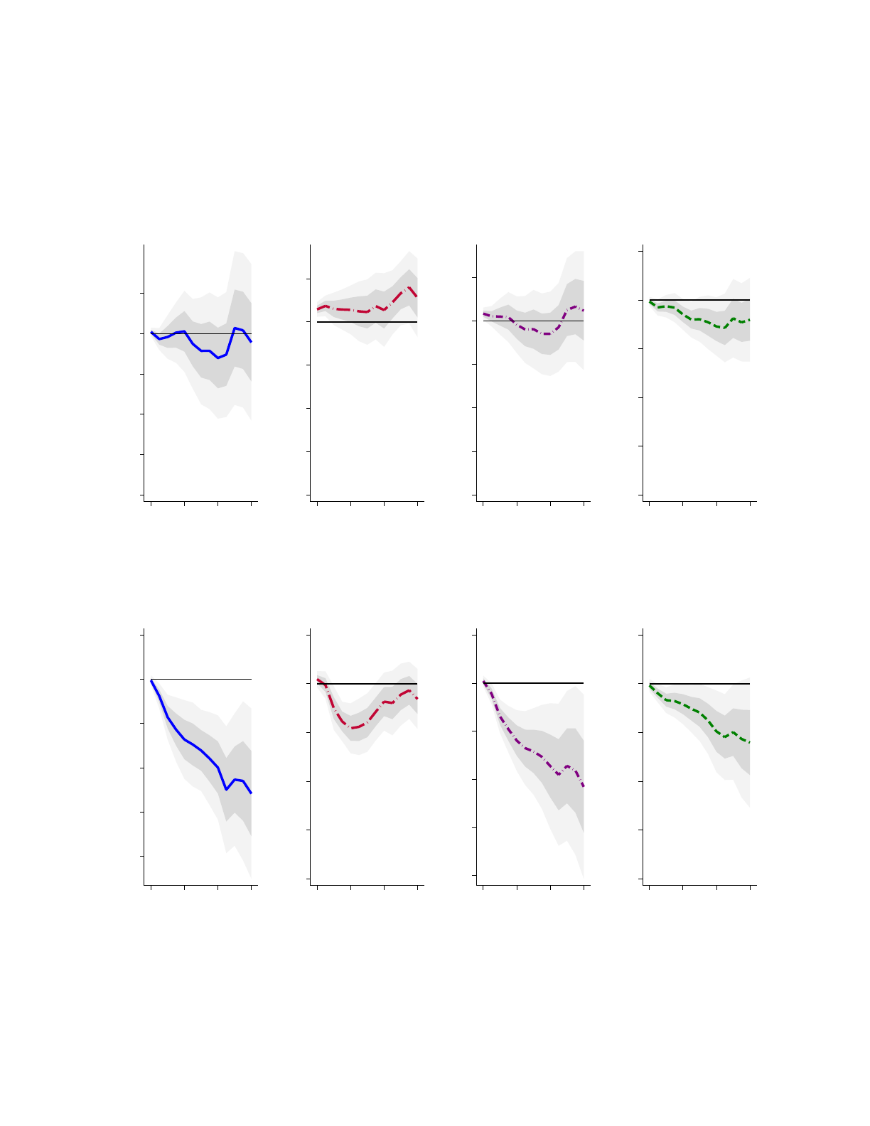
Figure 9:
Baseline asymmetric responses to 100 bps loosening and tightening shocks: Real GDP and
Solow decomposition. Full sample, 1900–2015.
(a) Estimates using Imbs correction for factor utilization, loosening shock
-8 -6 -4 -2 0 2
Percent
0 4 8 12
Year
Real GDP
-8 -6 -4 -2 0 2
Percent
0 4 8 12
Year
Labor
-8 -6 -4 -2 0 2
Percent
0 4 8 12
Year
Capital
-8 -6 -4 -2 0 2
Percent
0 4 8 12
Year
TFP
(b) Estimates using Imbs correction for factor utilization, tightening shock
-8 -6 -4 -2 0 2
Percent
0 4 8 12
Year
Real GDP
-8 -6 -4 -2 0 2
Percent
0 4 8 12
Year
Labor
-8 -6 -4 -2 0 2
Percent
0 4 8 12
Year
Capital
-8 -6 -4 -2 0 2
Percent
0 4 8 12
Year
TFP
Notes: Response to a 100 bps loosening and tightening shock in domestic short-term interest rate instrumented with the trilemma
IVs. Full sample: 1900–2015 (World Wars excluded). LP-IV estimates displayed as a thick lines with 68% and 95% standard error
bands. Both panels adjusts the raw data on capital stock and total hours to obtain estimates of actual factor inputs by using
the Imbs (1999) correction. In the upper panel the instrument
z
is replaced with zero when
z >
0 or ∆
R >
0, to include only
loosening shocks. In the lower panel the instrument
z
is replaced with zero when
z <
0 or ∆
R <
0,to include only tightening shocks.
Estimation is robust with Driscoll and Kraay (1998) standard errors. See text.
32

It is therefore natural to explore whether such symmetries appear at the longer 10+ year
horizon that we study here. Figure 9 presents some additional findings in this regard for our
baseline, full-sample, Solow decomposition responses. In the upper panel, the trilemma shocks
are restricted to include only strict loosening shocks: the instrument
z
is replaced with zero
when
z >
0 or ∆
R >
0, so both the shock in the foreign base and the rate change in the home
peg move in a negative direction. In the lower panel, the trilemma shocks are restricted to
include only strict tightening shocks: the instrument
z
is replaced with zero when
z <
0 or
∆
R <
0, so both the shock in the foreign base and the rate change in the home peg move in a
positive direction.
For loosening shocks in Figure 9a, we see that, relative to baseline, any strong evidence for
hysteresis virtually disappears. None of the responses is negative and statistically significant
at long horizons, although some of the point estimates still go in the same direction. For
tightening shocks in Figure 9b, we see that relative to baseline, the evidence for hysteresis is
even stronger. All of the responses are negative and statistically significant at long horizons,
larger than in the baseline, and clearly this is what was driving our main result.
The lesson of this exercise highlights a plausible, but important caveat to our main results.
Central banks can’t manipulate the supply-side of the economy to increase its long-run capacity
by exploiting loose policy. However, when policy is kept too tight, monetary policy can decrease
the long-run productive capacity of the economy. This evidence of asymmetric hysteresis
therefore carries important lessons for policy. The balance of risks for monetary policy mistakes
are not evenly weighted when it comes to the long-run productive path of the economy:
unusually tight policy risks significant downside damage, but unusually loose policy can’t do
much to deliver any upside benefit.
7. Real Effects of Monetary Shocks in the Literature
We now briefly compare our finding of persistent effects of monetary shocks to the literature.
We find that, when we extend the estimation horizon, some of the recent prominent studies in
this literature yield reassuringly similar findings of longer-run non-neutrality, even though the
main focus of these studies was quite different and looked at a shorter horizon. These results
for U.S. and U.K. economies in recent periods is consistent with relatively long-lived effects of
monetary policy across different identification schemes.
In Figures 10–12, we replicate and extend estimates from the published studies of Miranda-
Agrippino and Ricco (2021) and Brunnermeier, Palia, Sastry, and Sims (2021) for the U.S.
economy, and Cesa-Bianchi, Thwaites, and Vicondoa (2020) for the U.K. economy. Using their
published replication codes, we increase estimation horizon to 8-years or 96-months.
33

Figure 10: Effects of monetary shocks in the U.S., Miranda-Agrippino and Ricco (2021)
(a) Industrial Production
-2.5 -2 -1.5 -1 -.5 0
Percent
0 24 48 72 96
Months
(b) One-year T-bond
-.5 0 .5 1
Percent
0 24 48 72 96
Months
Notes: The figure plots the estimated IRFs for U.S. Industrial Production and One-year Treasury Bond to monetary policy shocks.
Panels (a) and (b) display our estimates from a Bayesian VAR(12) on monthly data (1979:1–2014:12) using Miranda-Agrippino and
Ricco (2021, Figure 3)’s informationally robust monetary policy instruments. IRFs are traced following a one-time exogenous shock
in the interest rate of about 100 basis points. Shaded areas denote 90% posterior coverage bands in panels (a) and (b).
Miranda-Agrippino and Ricco (2021) estimate a six-variable monthly Bayesian VAR(12)
for the U.S. economy with high-frequency market-based monetary surprises around Federal
Open Market Committee announcements following the work of G¨urkaynak, Sack, and Swanson
(2005).
24
They propose an identification strategy that makes use of Greenbook forecasts to
control for the central bank’s information set. They label their instrument as informationally
robust monetary policy instrument (MPI). Figure 10 reports impulse responses estimated from
using the methodology reported in their Figure 3. The shock is normalized to induce a 100
basis points increase in the one-year rate. Shaded areas denote 90% posterior coverage bands
in both panels.
Brunnermeier, Palia, Sastry, and Sims (2021) estimate a ten-variable monthly Bayesian
SVAR(10) model identified by heteroskedasticity (Rigobon, 2003) to study the relationship
between credit, output, and monetary policy.
25
Using time-varying variance across historical
episodes in the U.S. economy from the 1970s, they identify monetary policy shocks. Figure 11
reports impulse responses using their replication code for column 1 of their Figures 1 through
4. The shock is scaled to draws from a unit-scale
t
distribution with 5.7 degrees of freedom.
Shaded areas denote 90% posterior coverage bands in both panels.
24
Their Bayesian VAR is based on work by Coibion (2012) and Gertler and Karadi (2015). The vector
includes industrial production, the unemployment rate, the consumer price index, a commodity price index, the
excess bond premium of Gilchrist and Zakrajˇsek (2012), and the one-year nominal rate as the policy rate.
25
The vector includes industrial production, personal consumption expenditure price index, sum of commercial
bank real estate and consumer loans, commercial bank commercial & industrial loans, M1 money supply, Federal
funds rate, a commodity price index, term spread of 10 year over 3 month Treasuries, Gilchrist and Zakrajˇsek
(2012)’s bond spread, and “TED spread” of 3-month Eurodollars over 3 month Treasuries.
34

Figure 11: Effects of monetary shocks in the U.S., Brunnermeier et al. (2021)
(a) Industrial Production
-4 -3 -2 -1 0 1
Percent
0 24 48 72 96
Months
(b) Fed Funds Rate
-.5 0 .5 1 1.5
Percent
0 24 48 72 96
Months
Notes: The figure plots the estimated IRFs for U.S. Industrial Production and Effective Federal Funds Rate to monetary
policy shocks. Panels (a) and (b) display estimates from a large-scale Bayesian VAR with heteroskedasticity on monthly data
(1973:1–2015:6) from Brunnermeier et al. (2021). IRFs are traced following a one-time exogenous shock in the interest rate of
about 40 basis points. Shaded areas denote 90% posterior coverage bands in panels (a) and (b).
Figure 12: Effects of monetary shocks in the U.K., Cesa-Bianchi et al. (2020)
(a) Monthly estimate of GDP
-3 -2 -1 0 1
Percent
0 24 48 72 96
Months
(b) One-year Gilt Rate
-.5 0 .5 1 1.5
Percent
0 24 48 72 96
Months
Notes: Extended estimates from Figures 2 and 3 from high-frequency identification of U.K. monetary shocks Cesa-Bianchi, Thwaites,
and Vicondoa (2020). Shaded areas denote 68% confidence intervals computed using moving block bootstrap with 5,000 replications.
Sample: 1992:1–2015:1.
35

Cesa-Bianchi, Thwaites, and Vicondoa (2020) estimate a monthly SVAR with external
instruments following Mertens and Ravn (2013) and Gertler and Karadi (2015). They construct
a new series of monetary policy surprises for the U.K. using intra-day data on the price of three-
month Sterling futures contracts around announcements by the Monetary Policy Committee of
the Bank of England.
26
Figure 12 reports impulse responses estimated using the methodology
in their Figure 3. The shock is normalized to induce a 100 basis points increase in the one-year
rate. Shaded areas denote 68% confidence intervals computed using moving block bootstrap
with 5,000 replications (Jentsch and Lunsford, 2019).
Based on just three recent papers, these figures show strikingly persistent response of output
to transitory monetary interventions. But evidence consistent with our findings can also be
found in a range of other studies in the literature. As noted in the introduction, Bernanke
and Mihov (1998) also found similar persistent real effects. We report a screenshot of their
results in Figure A2 in the appendix. Moran and Queralto (2018) estimate a causal effect
of monetary policy shocks on TFP growth using a three-equation VAR model and Cholesky
identification for the U.S. economy. Plagborg-Møller (2019) finds long-run effects of monetary
shocks using Bayesian inference on Structural Vector Moving Average representation of the U.S.
data. Willems (2020) documents persistent effects of large monetary tightenings in a panel
data spanning 162 countries over 1970–2017. Palma (2022) shows exogenous increases in money
supply in the early modern period had a persistent effect of real activity. Cloyne and H¨urtgen
(2014, Fig 3), in their Bank of England working paper, document very persistent real effects
of monetary shocks in the U.K. economy using an auto-regressive distributed lag framework,
also used by Romer and Romer (2004). Cloyne and H¨urtgen (2014) find that the dynamics
of the underlying shock process play an important role in recovering long-run effects in their
estimation method. In a similar vein, McKay and Wieland (2021) document a boom-bust cycle
to the narrative monetary shocks series of Romer and Romer (2004), but in that setting the
interest-rate tightening cycle is followed by an easing cycle in their estimation. A rationalization
of heterogeneity in estimated responses was offered by Coibion (2012) who demonstrated that
different estimations of causal effects of monetary shocks may produce different results as the
underlying shock process vary in terms of size and persistence.
26
The vector includes the consumer price index, the unemployment rate, the nominal effective exchange rate,
the mortgage and corporate bond spreads, the nominal yield on the 1-year gilt as the policy rate, the spread
between the Moody’s BAA corporate bond and the U.S. 10-year government bond, a monthly estimate of GDP,
a measure of credit quantities, equity prices, and the trade balance. The policy surprises are available from
1997:6 to 2015:1. They use two lags in their VAR, we report results from a four lag specification to allow more
persistence following the econometric lessons from section 4. Estimates from VAR(2) are also persistent, but
produce a relatively sharper recovery to zero.
36

8. Conclusion
This paper challenges the view that money is neutral in the long-run. We find that monetary
policy has real effects that last for a decade or more. In an important caveat, we find responses
are asymmetric: strong for a tightening shock, weak for a loosening shock. We spent considerable
time and energy with the three pillars of our empirical strategy—identification, data, and
methods—to assure the reader that our results are solid.
The source of the main hysteresis result—that monetary policy shocks have long-lasting
effects on output—was striking to us even though a careful read of the literature suggests
that the evidence had been mounting for years. We find that capital and TFP growth are
the main drivers of this result, but not hours worked, in contrast to standard models of labor
hysteresis. Eventually the labor market returns to its pre-shock datum, but the levels of capital
and TFP remain scarred. Our findings do not negate the influence of labor frictions in shaping
the business cycle at shorter horizons. Instead, after a few years, we do not find a strong role
for such labor scarring in explaining why monetary policy has such long-lived effects.
There is much that is left unexplored in this paper as it is already quite long. Determining the
micro-foundations that explain TFP growth hysteresis would require a different paper devoted
to the topic with a completely different data set. Exploring the optimality of the monetary
policy rule in more general settings, and the welfare consequences of the hysteresis results
documented here are of first order importance for policymakers. Perhaps more importantly,
our paper challenges long-held views that require a reexamination of standard business cycle
models and evidence.
37

References
Akerlof, George A., William T. Dickens, and George L. Perry. 1996. The Macroeconomics of Low
Inflation. Brookings Papers on Economic Activity 1996(1): 1–76.
Angrist, Joshua D.,
`
Oscar Jord`a, and Guido M. Kuersteiner. 2018. Semiparametric Estimates of
Monetary Policy Effects: String Theory Revisited. Journal of Business and Economic Statistics
36(3): 371–387.
Antolin-Diaz, Juan, and Paolo Surico. 2022. The Long-Run Effects of Government Spending. CEPR
Discussion Paper DP17433.
Anzoategui, Diego, Diego Com´ın, Mark Gertler, and Joseba Mart´ınez. 2019. Endogenous Technology
Adoption and R&D as Sources of Business Cycle Persistence. American Economic Journal:
Macroeconomics 11(3): 67–110.
Bai, Jushan, and Pierre Perron. 1998. Estimating and Testing Linear Models with Multiple Structural
Changes. Econometrica 66(1): 47–78.
Baqaee, David Rezza, and Emmanuel Farhi. 2019. Productivity and Misallocation in General
Equilibrium. Quarterly Journal of Economics 135(1): 105–163.
Barlevy, Gadi. 2004. The Cost of Business Cycles under Endogenous Growth. American Economic
Review 94(4): 964–990.
Barnichon, Regis, Davide Debortoli, and Christian Matthes. 2021. Understanding the Size of the
Government Spending Multiplier: It’s in the Sign. Review of Economic Studies 89(1): 87–117.
Basu, Susanto, and John G Fernald. 2002. Aggregate Productivity and Aggregate Eechnology.
European Economic Review 46(6): 963–991.
Basu, Susanto, John G. Fernald, and Miles S. Kimball. 2006. Are Technology Improvements Contrac-
tionary? American Economic Review 96(5): 1418–1448.
Basu, Susanto, and Miles S. Kimball. 1997. Cyclical Productivity with Unobserved Input Variation.
NBER Working Paper 5915.
Benigno, Gianluca, and Pierpaolo Benigno. 2003. Price Stability in Open Economies. Review of
Economic Studies 70(4): 743–764.
Benigno, Gianluca, and Luca Fornaro. 2018. Stagnation Traps. Review of Economic Studies 85(3):
1425–1470.
Benigno, Gianluca, Luca Fornaro, and Martin Wolf. 2020. The Global Financial Resource Curse.
Federal Reserve Bank of New York Staff Report 915.
Benigno, Pierpaolo, and Luca Antonio Ricci. 2011. The Inflation-Output Trade-off with Downward
Wage Rigidities. American Economic Review 101(4): 1436–66.
Benigno, Pierpaolo, and Michael Woodford. 2012. Linear-Quadratic Approximation of Optimal Policy
Problems. Journal of Economic Theory 147(1): 1–42.
38

Bergeaud, Antonin, Gilbert Cette, and R´emy Lecat. 2016. Productivity Trends in Advanced Countries
between 1890 and 2012. Review of Income and Wealth 62(3): 420–444.
Berk, Kenneth N. 1974. Consistent autoregressive spectral estimates. Annals of Statistics 2(3):
489–502.
Bernanke, Ben S., and Ilian Mihov. 1998. The Liquidity Effect and Long-run Neutrality. Carnegie-
Rochester Conference Series on Public Policy 49(1): 149–194.
Bianchi, Francesco, Howard Kung, and Gonzalo Morales. 2019. Growth, Slowdowns, and Recoveries.
Journal of Monetary Economics 101(C): 47–63.
Bianchi, Javier, and Guido Lorenzoni. 2022. The prudential use of capital controls and foreign currency
reserves. In Handbook of International Economics: International Macroeconomics, Volume 6, edited
by Gopinath, Gita, Elhanan Helpman, and Kenneth Rogoff, 237–289. Elsevier.
Bianchi, Javier, Pablo Ottonello, and Ignacio Presno. Forthcoming. Fiscal Stimulus under Sovereign
Risk. Journal of Political Economy .
Blanchard, Olivier. 2018. Should We Reject the Natural Rate Hypothesis? Journal of Economic
Perspectives 32(1): 97–120.
Blanchard, Olivier J., and Lawrence H. Summers. 1986. Hysteresis and the European Unemployment
Problem. In NBER Macroeconomics Annual 1986, volume 1, 15–90. Cambridge, Mass.: MIT Press.
Blanchard, Olivier Jean, and Charles M. Kahn. 1980. The Solution of Linear Difference Models under
Rational Expectations. Econometrica 48(5): 1305–1311.
Born, Benjamin, Francesco D’Ascanio, Gernot J M¨uller, and Johannes Pfeifer. 2022. Mr. Keynes
meets the Classics: Government spending and the Real Exchange Rate. CEPR Discussion Paper
DP14073.
Brunnermeier, Markus, Darius Palia, Karthik A. Sastry, and Christopher A. Sims. 2021. Feedbacks:
Financial Markets and Economic Activity. American Economic Review 111(6): 1845–79.
Calvo, Guillermo A. 1983. Staggered Prices in a Utility-maximizing Framework. Journal of Monetary
Economics 12(3): 383–398.
Cerra, Valerie, Antonio Fat´as, and Sweta C. Saxena. 2023. Hysteresis and Business Cycles. Journal
of Economic Literature 61(1): 181–225.
Cesa-Bianchi, Ambrogio, Gregory Thwaites, and Alejandro Vicondoa. 2020. Monetary Policy Trans-
mission in the United Kingdom: A High Frequency Identification Approach. European Economic
Review 123: 103375.
Christiano, Lawrence. 2015. Applications of DSGE Model: What Happens if we Switch from Fixed to
Flexible Interest Rate Regime? Northwestern University. Unpublished.
Christiano, Lawrence J., Martin Eichenbaum, and Charles L. Evans. 1999. Monetary Policy Shocks:
What Have We Learned and To What End? In Handbook of Macroeconomics, edited by John
B. Taylor and Michael Woodford, volume 1 of Handbook of Macroeconomics, chapter 2, 65–148.
Amsterdam: Elsevier.
39

Cloyne, James, and Patrick H¨urtgen. 2014. The Macroeconomic Effects of Monetary Policy: A New
Measure for the United Kingdom. Bank of England Working Paper 493.
Cloyne, James, Joseba Mart´ınez, Haroon Mumtaz, and Paolo Surico. 2022. Short-Term Tax Cuts,
Long-Term Stimulus. NBER Working Paper 30246.
Coibion, Olivier. 2012. Are the effects of monetary policy shocks big or small? American Economic
Journal: Macroeconomics 4(2): 1–32.
Conley, Timothy G., Christian B. Hansen, and Peter E. Rossi. 2012. Plausibly Exogenous. Review of
Economics and Statistics 94(1): 260–272.
di Giovanni, Julian, Justin McCrary, and Till Von Wachter. 2009. Following Germany’s lead: Using
international monetary linkages to estimate the effect of monetary policy on the economy. Review
of Economics and Statistics 91(2): 315–331.
Driscoll, John C., and Aart C. Kraay. 1998. Consistent covariance matrix estimation with spatially
dependent panel data. Review of Economics and Statisticsfor 80(4): 549–560.
Durbin, J. 1959. Efficient Estimation of Parameters in Moving-Average Models. Biometrika 46(3/4):
306–316.
Eggertsson, Gauti B., and Michael Woodford. 2003. The Zero Bound on Interest Rates and Optimal
Monetary Policy. Brookings Papers on Economic Activity 2003(1): 139–211.
Farhi, Emmanuel, and Iv´an Werning. 2012. Dealing with the Trilemma: Optimal Capital Controls
with Fixed Exchange Rates. NBER Working Paper 18199.
Farhi, Emmanuel, and Iv´an Werning. 2017. Fiscal Unions. American Economic Review 107(12):
3788–3834.
Fat´as, Antonio. 2000. Do business cycles cast long shadows? Short-run persistence and economic
growth. Journal of Economic Growth 5(2): 147–162.
Fernald, John G. 2014. A quarterly, utilization-adjusted series on total factor productivity. Federal
Reserve Bank of San Francisco Working Paper 2012-19.
Fornaro, Luca. 2015. Financial crises and exchange rate policy. Journal of International Economics
95(2): 202–215.
Fornaro, Luca, and Federica Romei. 2019. The Paradox of Global Thrift. American Economic Review
109(11): 3745–79.
Fornaro, Luca, and Martin Wolf. 2022. The Scars of Supply Shocks: Implications for Monetary Policy.
CEPR Discussion Paper 15423.
Furlanetto, Francesco, Antoine Lepetit, Ørjan Robstad, Juan Rubio-Ram´ırez, and P˚al Ulvedal. 2021.
Estimating hysteresis effects. Norges Bank Working Paper 2020/13.
Gal´ı, Jordi. 1998. The liquidity effect and long-run neutrality: A comment. Carnegie-Rochester
Conference Series on Public Policy 49: 195–206.
Gal´ı, Jordi. 2015a. Hysteresis and the European Unemployment Problem Revisited. NBER Working
Paper 21430.
40

Gal´ı, Jordi. 2015b. Monetary policy, inflation, and the business cycle: An introduction to the new
Keynesian framework and its applications. Princeton, N.J.: Princeton University Press.
Gal´ı, Jordi. 2020. Insider-Outsider Labor Markets, Hysteresis and Monetary Policy. NBER Working
Paper 27385.
Gal´ı, Jord´ı, and Tommaso Monacelli. 2016. Understanding the Gains from Wage Flexibility: The
Exchange Rate Connection. American Economic Review 106(12): 3829–68.
Garga, Vaishali, and Sanjay R. Singh. 2021. Output Hysteresis and Optimal Monetary Policy. Journal
of Monetary Economics 117: 871–886.
Gertler, Mark, and Peter Karadi. 2015. Monetary Policy Surprises, Credit Costs, and Economic
Activity. American Economic Journal: Macroeconomics 7(1): 44–76.
Gilchrist, Simon, and Egon Zakrajˇsek. 2012. Credit spreads and business cycle fluctuations. American
Economic Review 102(4): 1692–1720.
Gordon, Robert J. 2016. The Rise and Fall of American Growth: The U.S. Standard of Living since
the Civil War. Princeton, N.J.: Princeton University Press.
Gourinchas, Pierre-Olivier. 2018. Monetary Policy Transmission in Emerging Markets: An Application
to Chile. In Monetary Policy and Global Spillovers: Mechanisms, Effects and Policy Measures,
edited by Enrique G. Mendoza, Ernesto Past´en, and Diego Saravia, volume 25 of Central Banking,
Analysis, and Economic Policies Book Series, chapter 8, 279–324. Santiago: Central Bank of Chile.
Guerrieri, Luca, and Matteo Iacoviello. 2015. OccBin: A toolkit for solving dynamic models with
occasionally binding constraints easily. Journal of Monetary Economics 70: 22–38.
Guerron-Quintana, Pablo A., and Ryo Jinnai. 2019. Financial frictions, trends, and the great recession.
Quantitative Economics 10(2): 735–773.
G¨urkaynak, Refet S, Brian Sack, and Eric Swanson. 2005. Do Actions Speak Louder Than Words?
The Response of Asset Prices to Monetary Policy Actions and Statements. International Journal
of Central Banking 1(1): 55–94.
Hume, David. 1752. ‘Of Money’, ‘Of Interest’ and ‘Of the Balance of Trade’. In Essays Moral, Political,
and Literary, edited by Eugene F. Miller. Indianapolis, Ind.: Liberty Fund.
Ilzetzki, Ethan, Carmen M. Reinhart, and Kenneth S. Rogoff. 2019. Exchange Arrangements Entering
the Twenty-First Century: Which Anchor will Hold? Quarterly Journal of Economics 134(2):
599–646.
Imbs, Jean M. 1999. Technology, growth and the business cycle. Journal of Monetary Economics
44(1): 65–80.
Jentsch, Carsten, and Kurt G Lunsford. 2019. The dynamic effects of personal and corporate income
tax changes in the United States: Comment. American Economic Review 109(7): 2655–78.
Jord`a,
`
Oscar. 2005. Estimation and Inference of Impulse Responses by Local Projections. American
Economic Review 95(1): 161–182.
41

Jord`a,
`
Oscar, Moritz Schularick, and Alan M. Taylor. 2016. The great mortgaging: housing finance,
crises and business cycles. Economic Policy 31(85): 107–152.
Jord`a,
`
Oscar, Moritz Schularick, and Alan M. Taylor. 2017. Macrofinancial History and the New
Business Cycle Facts. NBER Macroeconomics Annual 31(1): 213–263.
Jord`a,
`
Oscar, Moritz Schularick, and Alan M. Taylor. 2020. The effects of quasi-random monetary
experiments. Journal of Monetary Economics 112: 22–40.
Kilian, Lutz. 1998. Small-sample Confidence Intervals for Impulse Response Functions. Review of
Economics and Statistics 80(2): 218–230.
King, Robert G., and Mark W. Watson. 1997. Testing Long-Run Neutrality. Federal Reserve Bank of
Richmond Economic Quarterly 83(3): 69–101.
Kuersteiner, Guido M. 2005. Automatic Inference For Infinite Order Vector Autoregressions. Econo-
metric Theory 21(1): 85–115.
Las´een, Stefan, and Lars E. O. Svensson. 2011. Anticipated Alternative Policy Rate Paths in Policy
Simulations. International Journal of Central Banking 7(3): 1–35.
Lewis, Richard, and Gregory C. Reinsel. 1985. Prediction of multivariate time series by autoregressive
model fitting. Journal of Multivariate Analysis 16(3): 393–411.
Li, Dake, Mikkel Plagborg-Møller, and Christian K Wolf. 2022. Local Projections vs. VARs: Lessons
From Thousands of DGPs. NBER Working Paper 30207.
Lusompa, Amaze B. 2019. Local projections, autocorrelation, and efficiency. UC Irvine. Unpublished.
Mankiw, N. Gregory. 2001. The inexorable and mysterious tradeoff between inflation and unemployment.
Economic Journal 111(471): 45–61.
McKay, Alisdair, and Johannes F. Wieland. 2021. Lumpy Durable Consumption Demand and the
Limited Ammunition of Monetary Policy. Econometrica 89(6): 2717–2749.
Meier, Matthias, and Timo Reinelt. Forthcoming. Monetary Policy, Markup Dispersion, and Aggregate
TFP. Review of Economics and Statistics .
Mertens, Karel, and Morten O. Ravn. 2013. The Dynamic Effects of Personal and Corporate Income
Tax Changes in the United States. American Economic Review 103(4): 1212–1247.
Miranda-Agrippino, Silvia, and Giovanni Ricco. 2021. The transmission of monetary policy shocks.
American Economic Journal: Macroeconomics 13(3): 74–107.
Montiel Olea, Jos´e Luis, and Mikkel Plagborg-Møller. 2021. Local Projection Inference Is Simpler and
More Robust Than You Think. Econometrica 89(4): 1789–1823.
Moran, Patrick, and Albert Queralto. 2018. Innovation, productivity, and monetary policy. Journal
of Monetary Economics 93: 24–41.
Nakamura, Emi, and J´on Steinsson. 2018. Identification in Macroeconomics. Journal of Economic
Perspectives 32(3): 59–86.
42

Obstfeld, Maurice, and Kenneth Rogoff. 1995a. Exchange rate dynamics redux. Journal of Political
Economy 103(3): 624–660.
Obstfeld, Maurice, and Kenneth Rogoff. 1995b. The Mirage of Fixed Exchange Rates. Journal of
Economic Perspectives 9(4): 73–96.
Obstfeld, Maurice, Jay C. Shambaugh, and Alan M. Taylor. 2004. Monetary sovereignty, exchange
rates, and capital controls: The trilemma in the interwar period. IMF Staff Papers 51(S1): 75–108.
Obstfeld, Maurice, Jay C. Shambaugh, and Alan M. Taylor. 2005. The Trilemma in History: Tradeoffs
Among Exchange Rates, Monetary Policies, and Capital Mobility. Review of Economics and
Statistics 87(3): 423–438.
Palma, Nuno. 2022. The real effects of monetary expansions: evidence from a large-scale historical
experiment. Review of Economic Studies 89(3): 1593–1627.
Plagborg-Møller, Mikkel. 2019. Bayesian inference on structural impulse response functions. Quanti-
tative Economics 10(1): 145–184.
Plagborg-Møller, Mikkel, and Christian K Wolf. 2021. Local projections and VARs estimate the same
impulse responses. Econometrica 89(2): 955–980.
Queralto, Albert. 2020. A model of slow recoveries from financial crises. Journal of Monetary
Economics 114: 1–25.
Quinn, Dennis, Martin Schindler, and A. Maria Toyoda. 2011. Assessing measures of financial openness
and integration. IMF Economic Review 59(3): 488–522.
Ramey, Valerie A. 2016. Macroeconomic Shocks and Their Propagation. In Handbook of Macroeco-
nomics, edited by John B. Taylor and Harald Uhlig, volume 2 of Handbook of Macroeconomics,
chapter 2, 71–162. Amsterdam: Elsevier.
Rigobon, Roberto. 2003. Identification through heteroskedasticity. Review of Economics and Statistics
85(4): 777–792.
Romer, Christina D., and David H. Romer. 2004. A New Measure of Monetary Shocks: Derivation
and Implications. American Economic Review 94(4): 1055–1084.
Schmitt-Groh´e, Stephanie, and Mart´ın Uribe. 2003. Closing small open economy models. Journal of
International Economics 61(1): 163–185.
Schmitt-Groh´e, Stephanie, and Mart´ın Uribe. 2016. Downward Nominal Wage Rigidity, Currency.
Pegs, and Involuntary Unemployment. Journal of Political Economy 124(5): 1466–1514.
Schmitt-Groh´e, Stephanie, Mart´ın Uribe, and Michael Woodford. 2022. International Macroeconomics:
A Modern Approach. Princeton, N.J.: Princeton University Press.
Schm¨oller, Michaela Elfsbacka, and Martin Spitzer. 2021. Deep recessions, slowing productivity and
missing (dis-)inflation in the euro area. European Economic Review 134: 103708.
Shambaugh, Jay C. 2004. The Effect of Fixed Exchange Rates on Monetary Policy. Quarterly Journal
of Economics 119(1): 301–352.
43

Stadler, George W. 1990. Business Cycle Models with Endogenous Technology. American Economic
Review 80(4): 763–78.
Syverson, Chad. 2011. What determines productivity? Journal of Economic Literature 49(2): 326–365.
Tenreyro, Silvana, and Gregory Thwaites. 2016. Pushing on a String: US Monetary Policy is Less
Powerful in Recessions. American Economic Journal: Macroeconomics 8(4): 43–74.
Uribe, Mart´ın, and Stephanie Schmitt-Groh´e. 2017. Open Economy Macroeconomics. Princeton, N.J.:
Princeton University Press.
Vinci, Francesca, and Omar Licandro. 2021. Switching-track after the Great Recession. CESifo
Working Paper 9107.
Werning, Iv´an. 2011. Managing a Liquidity Trap: Monetary and Fiscal Policy. NBER Working Paper
17344.
Willems, Tim. 2020. What do monetary contractions do? Evidence from large tightenings. Review of
Economic Dynamics 38: 41–58.
Xu, Ke-Li. 2023. Local Projection Based Inference under General Conditions. CAEPR Working
Papers 2023-001, Department of Economics, Indiana University Bloomington.
Yellen, Janet L. 2016. Macroeconomic Research After the Crisis. Speech at the conference “The
Elusive ‘Great’ Recovery: Causes and Implications for Future Business Cycle Dynamics,” Federal
Reserve Bank of Boston, October.
44

ONLINE APPENDIX
A. Equilibrium conditions in the baseline model
A perfect foresight equilibrium in the baseline model (subsection 2.3) is given by a sequence of
11 processes
{C
t
, C
T t
, C
Nt
, d
t+1
, R
t
, R
n
t
, l
t
, W
t
, P
T t
, E
t
, P
Nt
, }
that satisfy the following equilibrium
conditions for a given sequence of exogenous processes {Y
T t
, ε
t
, P
∗
t
} and initial values {d
1
},
C
t
=
C
T t
ω
ω
C
Nt
1 − ω
1−ω
, (31)
C
T t
+ d
t
= Y
T t
+
d
t+1
R
t
, (32)
C
−1
T t
= ζE
t
C
−1
T t+1
R
t
, (33)
R
t
= R
∗
t
, (34)
P
Nt
P
T t
=
(1 − ω)C
T t
ωC
Nt
, (35)
C
−1
T t
= ζE
t
(
C
−1
T t+1
R
n
t
P
T t+1
/P
T t
)
, (36)
φl
ν
t
C
T t
ω
=
W
t
P
T t
(37)
l
t
= C
Nt
(38)
P
T t
= E
t
P
∗
t
(39)
P
N1
=
¯
P
N
; and P
Nt
= W
t
∀t > 1 (40)
R
n
t
=
¯
R
n
e
ε
t
and R
∗
t
= ζ
−1
. (benchmark)
We label this the benchmark economy, and maintain it as is in exercises shown in Section 2.4
In the baseline peg economy configuration (subsection 2.4), equilibrium is given by the same
equations as above, except we replace the final equation with the following policy regime equation
(and shock process):
E
t
= 1 and R
∗
t
= ζ
−1
e
ε
t
(peg)
B. Solution for the baseline model and Proofs for Section 2
Notation To derive some of the results, we consider a first-order approximation of the equilibrium
conditions around the initial steady state (date 0 economy). For a variable
x
, we define:
ˆx
t
=
x
t
−¯x
¯x
.
In the case of d
t+1
, we define
ˆ
d
t+1
= d
t+1
−
¯
d.
B.1. Baseline model
We assume the economy starts in a flexible price steady state equilibrium indexed by initial debt
d
1
=
¯
d
. We set this initial external debt of the economy to zero,
¯
d
= 0. Real interest rates are equal
to inverse of the domestic discount factor:
R
t−1
=
R
∗
t−1
=
ζ
−1
, and tradable good consumption is
given by: C
T 0
= Y
T
. For tradable consumption to be positive, we assume
¯
d < Y
T
(1 − ζ)
−1
.
A1

World price of tradable good,
P
∗
t
, is normalized to one, and initial nominal exchange rate is
also normalized to one,
E
0
= 1. We normalize
φ
such that
l
=
L
N
=
C
N
= 1 in the steady
state. That is,
φ
= 1
− ω
. Real wages in units of tradables equal relative price of non-tradables:
W
/P
T
=
P
N
/P
T
=
1−ω
ω
Y
T
− (1 − ζ)
¯
d
.
There is a one-time unanticipated shock at date 1. In the peg configuration, the shock is to foreign
interest rate
R
∗
1
. In the benchmark configuration, the shock is to
ε
1
in the policy rule. The tradable
output endowment is constant at all dates: Y
T
.
We assume that non-tradable goods prices are pre-fixed to
1−ω
ω
Y
T
− (1 − ζ)
¯
d
for all non-tradable
firms at date 1. At future dates, non-tradable good prices are set flexibly to equal nominal wage
(marginal product of labor in domestic currency).
B.2. Proof for Proposition 1
Because of equal inter- and intra-temporal elasticities, loans market problem can be solved without
reference to labor market and non-tradable goods market.
Proof.
The proof follows directly from Equation 5, Equation 10, and Equation 13, which define the
competitive equilibrium for {C
T t
, R
t
, d
t+1
} a given sequence of {R
∗
t
}.
Date 2 onwards, the economy is in a steady state. The country’s external budget constraint at
dates 1 and 2:
C
T 1
= Y
T
− d
1
+
d
2
R
1
, (41)
C
T 2
= Y
T
− (1 − ζ)d
2
(42)
Combining the last two equations:
(1 − ζ) (C
T 1
− Y
T
+ d
1
) +
C
T 2
− Y
T
R
1
= 0
The demand for loans is given by :
d
2
ζR
1
=
Y
T
ζR
1
− (Y
T
− d
1
)
Home real interest rate is equal to the world real interest rate
R
t
= R
∗
t
Equilibrium is then
d
2
= (1 − ζR
∗
1
)Y
T
+ ζR
∗
1
d
1
Tradable good consumption is given by:
C
T 1
= Y
T
1 − ζ +
1
R
∗
1
− (1 − ζ) d
1
; C
T 2
= Y
T
ζ (R
∗
1
(1 − ζ) + 1) − (1 − ζ)ζR
∗
1
d
1
B.3. Proof for Proposition 2
Proof. Peg economy:
A2

Since
P
∗
t
is normalized to one, and nominal exchange rate is fixed (and normalized to one),
P
T t
= E
t
= P
∗
t
= 1.
We consider a one-time unanticipated increase in
ε
1
>
0. Hence,
C
T 1
=
Y
T
1 − ζ +
1
R
∗
1
−
(1 − ζ) d
1
< C
T 0
. Date 2 onwards, W
2
= P
N2
= p
2
=
(1−ω)C
T 2
ω
.
Non-tradable good production at date t falls below the steady state:
l
1
=
C
N1
=
C
T 1
C
T 0
<
1. To a
first order approximation,, and substituting
¯
d
= 0, non-tradable output in the benchmark economy is
given by
ˆ
l
1
=
ˆ
C
N1
= −ζε
1
.
where hats denote log-linear approximation around the initial steady state.
Benchmark economy:
There is a one-time unanticipated shock at date 1 to home nominal interest rate
R
n
1
=
ζ
−1
e
ε
1
, and
it returns to
R
n
2
=
ζ
−1
next period onwards. Consumption of tradable goods, debt and real interest
rate on tradable bond are not affected by this shock. Date 2 onwards, p
2
=
(1−ω)
ω
Y
T
− (1 − ζ)
¯
d
.
We can construct path for
{C
Nt
, P
Nt
, P
T t
}
that solves the system of equations such that
{C
Nt
}
is ex-
actly same as in the peg economy. Given the nominal rigidity,
P
T 1
=
E
1
=
C
N1
=
Y
T
1−ζ+
1
R
n
1
−(1−ζ)
¯
d
Y
T
−(1−ζ)
¯
d
.
From the consumption Euler equation for tradable good,
P
T 2
=
ζP
T 1
R
n
1
. Finally, we obtain
P
N2
=
(1−ω)
ω
Y
T
− (1 − ζ)
¯
d
P
T 2
.
The policy rule under a peg prevents any adjustment in nominal exchange rates, i.e.,
E
2
=
E
1
.
Hence the path of nominal interest rates in a peg economy,
R
n
t
, is identical to the path in the
benchmark economy for a given shock.
To a first order approximation, and substituting
¯
d
= 0, non-tradable output in the benchmark
economy is given by
ˆ
l
1
=
ˆ
C
N1
= −ζε
1
.
where hats denote log-linear approximation around the initial steady state.
Since the tradable output is an exogenous endowment, and we have assumed constant aggregation
weights, the impact-response of real GDP is identical across the two economies.
B.4. Proof of Proposition 3
Proof.
From interest rate Euler equation, and fixed foreign tradable prices, we obtain the interest
parity relationship between home rate and foreign rate
R
n
t
= R
∗
t
E
t+1
E
t
In an imperfect pass-through economy, after log-linearizing around initial steady state, we can write
ˆ
R
n
t
= λ
ˆ
R
∗
t
; λ ∈ (0, 1] . (43)
the expected exchange rate appreciation is now (1
− λ
)
ˆ
R
∗
t
. With same steps as in the proof provided
in subsection B.3, we obtain Proposition 3.
A3

B.5. Proof of Proposition 4
Proof.
The solution for benchmark economy is as discussed in subsection B.3. In the peg economy,
there is now endogenous production of tradables. Because of common labor markets and constant
returns to scale production in tradable good sector, real wages (in units of tradable goods) are equal
to one. Because the total labor supplied in the economy is divided between tradable and non-tradable
good sector, the labor market clearing condition is now modified as:
l
t
= L
T t
+ L
Nt
Substituting this market clearing condition in the intra-temporal labor supply condition of the
household, we get:
φ (L
T t
+ L
Nt
)
ν
C
T t
ω
= 1
We solve for the steady state value such that
L
T
=
¯
Y
T
>
0 and
L
N
=
C
N
= 1. From the
intra-temporal condition on choice between tradables and nontradables, we then get the steady state
tradable output:
¯
Y
T
=
ω
1 − ω
+ (1 − ζ)
¯
d
Tradable consumption is
ω
1−ω
. Finally, the labor disutility parameter is set such that labor market
clears:
φ =
1 − ω
¯
Y
T
+ 1
ν
Total labor employed in the initial steady state (indexed with
¯
d) is thus
¯
L = 1 +
ω
1 − ω
+ (1 − ζ)
¯
d
We assume that
¯
d = 0.
Because of the assumed nominal rigidity, tradables and non-tradables consumption co-move one
to one. As a result, the intra-temporal labor supply condition becomes
φ
Y
T t
+
ω
1−ω
C
T t
ν
C
T t
ω
= 1
Since
ν >
0, tradable output co-moves negatively with tradable (and non-tradable) consumption, and
tradable output is more volatile than non-tradable output.
From the following system of equations, we can find the solution for {C
T t
, Y
T t
, R
t
, d
t+1
, C
Nt
}
C
T t
+ d
t
= Y
T t
+
d
t+1
R
t
, (44)
C
−1
T t
= ζE
t
C
−1
T t+1
R
t
, (45)
R
t
= R
∗
t
(46)
1 =
φ
Y
T t
+
ω
1−ω
C
T t
ν
C
T t
ω
(47)
C
Nt
=
ω
1 − ω
C
T t
(48)
As before, the solution takes the following form: date 2 onwards the economy is in a new long-run.
A4

We log-linearize the equilibrium around the initial steady state to analytically derive the sign of the
bias from trilemma identification upto a first-order approximation for small shocks and initial debt
equal to zero.
ˆ
C
T t
+
1
¯
Y
T
d
t
=
ˆ
Y
T t
+
ζ
¯
Y
T
d
t+1
, (49)
ˆ
C
T t
=
ˆ
C
T t+1
−
ˆ
R
t
, (50)
ˆ
R
t
=
ˆ
R
∗
t
(51)
ˆ
Y
T t
= −
(1 + ν(1 − ω))
νω
ˆ
C
T t
(52)
ˆ
C
Nt
=
ˆ
C
T t
(53)
where
¯
Y
T
≡
ω
1−ω
.
The date-1 solution for non-tradable output and tradable-outptut is given by:
ˆ
C
N1
=
ˆ
C
T 1
= −ζ
ˆ
R
1
< 0;
ˆ
Y
T 1
=
(1 + ν(1 − ω))
νω
ζ
ˆ
R
1
> 0
Tradable output goes up in response to a one-time increase in
ˆ
R
∗
1
in the peg economy. There is an
increase in labor supply in the tradable goods sector following a contraction in demand for labor in
the non-tradable sector.
While the impact response of non-tradable output is identical across the peg and the benchmark
economy, total output’s response at date 1 is biased upwards (i.e., towards zero, or smaller absolute
size) in the peg economy relative the benchmark economy.
B.6. Proof of Proposition 5
Proof.
The log-linear equilibrium (around initial steady state with zero debt) conditions for tradable-
goods consumption, output, and real interest rate are given by:
ˆ
C
T t
+
1
¯
Y
T
d
t
=
ˆ
Y
T t
+
ζ
¯
Y
T
d
t+1
, (54)
ˆ
C
T t
=
ˆ
C
T t+1
−
ˆ
R
t
, (55)
ˆ
R
t
=
ˆ
R
∗
t
(56)
ˆ
Y
T t
= −α
ˆ
R
∗
t
. (57)
where
¯
Y
T
≡
ω
1−ω
. We can solve these equations to derive the response of tradable consumption at
date 1:
ˆ
C
T 1
= −ζ
ˆ
R
∗
1
− α(1 − ζ)
ˆ
R
∗
t
Rest of the economy is same as studied in the baseline peg economy. Given the nominal rigidity
and fixed exchange rate regime, tradable and non-tradable consumption perfectly co-move:
ˆ
C
T 1
=
ˆ
C
N1
.
The non-tradable output in the peg economy falls more than in the benchmark economy. The difference
is equal to α(1 − ζ)
ˆ
R
∗
t
.
In the presence of the spillover, tradable output contracts with an increase in base interest rates,
while it is unaffected in the benchmark economy.
Using the construction of real GDP described in Section 2.3, we can compute the approximate
A5

difference in the impulse responses of real GDP as
ˆ
Y
peg
t
−
ˆ
Y
benchmark
t
=
P
T
Y
T
P Y
|{z}
tradable output
share in GDP
× (
ˆ
Y
peg
T t
−
ˆ
Y
benchmark
T t
) +
P
N
Y
N
P Y
| {z }
non-tradable output
share in GDP
× (
ˆ
Y
peg
Nt
−
ˆ
Y
benchmark
Nt
)
(58)
=
P
T
Y
T
P Y
α
ˆ
R
∗
t
+
P
N
Y
N
P Y
α(1 − ζ)
ˆ
R
∗
t
. (59)
Now we assume that the base shock equals the benchmark policy shock,
ˆ
R
∗
t
= ε
t
, so we have that
ˆ
Y
peg
t
R
∗
t
|{z}
≡γ
p
−
ˆ
Y
benchmark
t
ϵ
t
| {z }
≡β
=
P
T
Y
T
P Y
+ (1 − ζ)
P
N
Y
N
P Y
α .
Hence,
β = γ
p
−
P
T
Y
T
P Y
+ (1 − ζ)
P
N
Y
N
P Y
α . (60)
C. Extension: time-varying aggregation weights
We consider the more general extension of the baseline model (subsection 2.3) allowing for time-
variation in aggregation weights in the construction of total output. The consumption aggregator is :
C
t
= Ψ
C
ω
T t
C
1−ω
Nt
, where Ψ
≡ ω
−ω
(1
− ω
)
1−ω
is a scaling factor. This implies that domestic CPI is
given by
P
t
=
P
ω
T t
P
1−ω
Nt
. Total nominal output is
P
T t
Y
T t
+
P
Nt
Y
Nt
. Let total output be denoted with
Y
t
, and is given by:
Y
t
=
P
T t
Y
T t
+ P
Nt
Y
Nt
P
t
= p
ω−1
t
Y
T t
+ p
ω
t
Y
Nt
,
where p
t
≡
P
Nt
P
T t
. From the optimality conditions, we have that
p
t
=
(1 − ω)C
T t
ωC
Nt
.
In terms of log-deviations from steady state, total output is given by
ˆ
Y
t
=
(ω − 1)p
ω−1
+ ωp
ω
ˆ
C
T t
−
ˆ
Y
Nt
+
P
T
Y
T
P Y
ˆ
Y
T t
+
P
N
Y
N
P Y
ˆ
Y
Nt
.
When ω → 0 (tradable goods share is infinitesimally small),
ˆ
Y
t
= p
−1
ˆ
Y
Nt
−
ˆ
C
T t
+
P
T
Y
T
P Y
ˆ
Y
T t
+
P
N
Y
N
P Y
ˆ
Y
Nt
.
In the baseline model, with exogenous endowment of tradable goods,
ˆ
Y
t
= p
−1
ˆ
Y
Nt
−
ˆ
C
T t
+
P
N
Y
N
P Y
ˆ
Y
Nt
.
A6

Recall that
ˆ
Y
Nt
is identical across the peg and the benchmark economy as proved in Proposition
2. From results in Appendix B sequence of
ˆ
C
T t
<
0 under a peg and equal to 0 under benchmark
economy. Hence the response of total output under a peg is downward biased relative to that under
the benchmark economy.
D. Proofs of consistency for impulse responses
This section provides the basic ideas behind the proofs of consistency for truncated VARs and LPs
when the true DGP is an invertible MA(
∞
). The reader is referred to the references cited for additional
details.
D.1. Data generating process and main assumptions
Assume the data generating process for the m–dimensional vector process y
t
is:
y
t
=
∞
X
j=0
B
j
ϵ
t−j
; B
0
= I;
∞
X
j=0
||B
j
|| < ∞ , (61)
where
||B
j
||
2
=
tr
(
B
′
j
B
j
) and
B
(
z
) =
P
∞
j=0
B
j
z
j
such that
det{B
(
z
)
} ̸
= 0 for
|z| ≤
1
.
Under these
assumptions, this invertible M A(∞) can also be expressed as:
y
t
=
∞
X
j=1
A
j
y
t−j
+ ϵ
t
;
∞
X
j=1
||A
j
|| < ∞; det{A(z)} ̸= 0 for |z| ≤ 1 .
Further, we make assumptions 1–4 following Lewis and Reinsel (1985), and Lusompa (2019) (Kuer-
steiner (2005) makes somewhat stronger assumptions because he later derives testing procedures to
determine the optimal lag length). These assumptions are:
Assumption 1 {y
t
} is generated by Equation 61.
Assumption 2 E|ϵ
it
ϵ
jt
ϵ
kt
ϵ
lt
| ≤ γ
4
< ∞ for 1 ≤ i, j, k, l ≤ m.
Assumption 3 The truncation lag
p
is chosen as a function of the sample size
T
such that
p
2
/T → 0 as p, T → ∞.
Assumption 4 p is chosen as a function of T such that
p
1/2
∞
X
j=p+1
||A
j
|| → 0 as p, T → ∞.
Then, as discussed in the text, Lewis and Reinsel (1985) show:
||
ˆ
A
j
− A
j
||
p
−→ 0 as p, T → ∞.
This well-known result says that even when the data are generated by an infinite-order process, the
coefficients of the first
p
terms are consistently estimated. We show next that despite this result,
inconsistencies in the estimation of impulse responses can crop up.
A7

D.2. Potential sources of bias in truncated VARs
In finite samples, inconsistent estimates of the impulse response function can arise from at least two
sources that we now quantify: (1) the truncation lag is too short given Assumptions 1–4; and (2) the
truncation lag is appropriate, but the impulse response is calculated for periods that extend beyond
the truncation lag. To investigate the first source of inconsistency, rewrite the V AR(∞) as
y
t
=
k
X
j=1
A
j
y
t−j
+ u
t
,
u
t
=
p
X
j=k+1
A
j
y
t−j
+
∞
X
j=p+1
A
j
y
t−j
+ ϵ
t
,
where we assume
k < p
and
p
is the truncation lag that meets Assumptions 1–4 of the proof of
consistency. Hence rewrite the previous expression as
y
t
= A(k)X
k,t−1
+ u
t
; A(k) = (A
1
, . . . , A
k
); X
k,t−1
= (y
t−1
, . . . , y
t−k
)
′
.
The least-squares estimate of A(k) is therefore
ˆ
A(k) =
1
T − k
T
X
p
y
t
X
′
k,t−1
!
1
T − k
T
X
p
X
k,t−1
X
′
k,t−1
!
−1
.
Hence
ˆ
A(k) = A(k) +
1
T − k
T
X
p
u
t
X
′
k,t−1
!
1
T − k
T
X
p
X
k,t−1
X
′
k,t−1
!
−1
.
Given the three components of
u
t
, it is easy to see that the source of inconsistency in estimates of the
first k autoregressive terms will come from the component
1
T − k
T
X
p
p
X
j=k+1
A
j
y
t−j
X
′
k,t−1
1
T − k
T
X
p
X
k,t−1
X
′
k,t−1
!
−1
,
since the proof of consistency in Lewis and Reinsel (1985) shows that the other two terms vanish
asymptotically. The source of inconsistency can be quantified by noticing that
1
T − k
T
X
p
X
k,t−1
X
′
k,t−1
!
−1
→
Γ(0) Γ(1) · · · Γ(k)
Γ(1) Γ(0) · · · Γ(k − 1)
.
.
.
.
.
.
.
.
.
.
.
.
Γ(k) Γ(k − 1) · · · Γ(0)
−1
→ Γ
−1
k
,
as shown in Lewis and Reinsel (1985), where
E
(
y
t
y
′
t−j
) = Γ(
j
) and Γ(
−j
) = Γ(
j
)
′
. Hence, asymptoti-
cally, the source of inconsistency is
p
X
k+1
A
j
(Γ(j − 1), . . . , Γ(j − k)) Γ
−1
k
.
A8

However, even when the lag-length
p
is chosen to be sufficiently large, another source of bias can crop
up into the estimation of the impulse response. In particular, following Durbin (1959), we know that
B
h
= A
1
B
h−1
+ A
2
B
h−2
+ · · · + A
h−1
B
1
+ A
h
.
If the VAR is truncated at lag k, for k ≤ p, it is easy to see that the previous expression becomes
B
h
= A
1
B
h−1
+ A
2
B
h−2
+ · · · + A
k
B
k−h
+ A
k+1
B
k−h−1
+ · · · + A
h−1
B
1
+ A
h
|
{z }
remainder
.
and, hence,
||
ˆ
B
h
− B
h
|| = ||A
k+1
(
ˆ
B
k−h−1
− B
k−h−1
) + . . . + A
h−1
(
ˆ
B
1
− B
1
) + A
h
|| ̸→ 0 ,
since ||
ˆ
B
k+j
− B
k+j
|| for j ≥ 1 is not guaranteed to vanish asymptotically.
Next notice that the impulse response for horizons h > k will be estimated using the recursion
ˆ
B
k+j
=
ˆ
A
1
ˆ
B
k+j−1
+ . . . +
ˆ
A
k
ˆ
B
j
; j = 1, . . . , H .
Even if k = p, and hence ||
ˆ
A
j
|| → A
j
for j = 1, . . . , k, the fact remains that the remainder term
A
k+1
B
k−h−1
+ · · · + A
h−1
B
1
+ A
h
cumulates increasing sums of coefficients that are not estimated in the model. As the Monte Carlo
exercise showed earlier, the inconsistency at longer horizons tends to accumulate.
D.3. The consistency of the local projections estimator
In this section we use the same assumptions as in the previous section to establish the consistency of
the local projections estimator at any horizon.
Using the VAR(∞) representation of the DGP and recursive substitution, it is easy to see that
y
t+h
= B
h+1
y
t−1
+ {C
h+2
y
t−2
+ C
h+3
y
t−3
+ · · · } + ϵ
t+h
+ B
1
ϵ
t+h−1
+ ϵ
t
B
h
,
where
C
h+2
= B
h
A
1
+ · · · + B
1
A
h
+ A
h+1
,
C
h+3
= B
h
A
2
+ · · · + B
1
A
h+1
+ A
h+2
,
.
.
.
C
h+k
= B
h
A
k−1
+ · · · + B
1
A
h+k−2
+ A
h+k−1
.
Now, consider truncating the lag of the local projection at
k
=
p
, where
p
meets Assumptions 1–4 of
the Lewis and Reinsel (1985) consistency theorem discussed in the previous section.
Then the truncated local projection can be written as
y
t+h
= B
h+1
y
t−1
+ C
h+2
y
t−2
+ C
h+3
y
t−3
· · · + C
h+k
y
t−k
+ u
t+h
,
u
t+h
= ϵ
t+h
+ {B
1
ϵ
t+h−1
+ B
2
ϵ
t+h−2
+ · · · + B
h
ϵ
t
} + {C
h+k+1
y
t−k−1
+ C
h+k+2
y
t−k−2
+ · · · } .
A9

Let
D
= (
B
h
, C
h+2
, . . . , C
h+k
) and
X
t−1
= (
y
t−1
, . . . , y
t−k
)
′
as defined earlier but where the
subscript k is omitted here for simplicity. Then the local projection can be compactly written as
y
t+h
= DX
t−1
+ u
t+h
.
The least-squares estimate of D is simply
ˆ
D =
1
T − h − k
T −h
X
k
y
t+h
X
′
t−1
!
1
T − h − k
T −h
X
k
X
t−1
X
′
t−1
!
−1
,
from where consistency can be determined from the following expression
ˆ
D = D +
1
T − h − k
T −h
X
k
u
t+h
X
′
t−1
!
1
T − h − k
T −h
X
k
X
t−1
X
′
t−1
!
−1
.
Lewis and Reinsel (1985) show that
||
Γ
−1
k
||
1
is uniformly bounded where we use the fact that
||AB||
2
≤ ||A||
2
1
||B||
2
; as well as
||AB||
2
≤ ||A||
2
||B||
2
1
where
||C||
2
1
=
sup
l̸=0
l
′
C
′
Cl/l
′
l
, the largest
eigenvalue of C
′
C (see Wiener and Masani, 1958).
Now we turn our focus to the terms
1
T − h − k
T −h
X
k
u
t+h
X
′
t−1
=
1
T − h − k
T −h
X
k
(ϵ
t+h
+ B
1
ϵ
t+h−1
+ · · · + B
h
ϵ
t
)X
′
t−1
=
1
T − h − k
T −h
X
k
(C
h+k
y
t−k−1
+ C
h+k+1
y
t−k−2
+ · · · )X
′
t−1
.
It is easy to see that
1
T − h − k
T −h
X
k
ϵ
t+h
X
′
t−1
→ 0 ,
B
j
T − h − k
T −h
X
k
ϵ
t+h−j
X
′
t−1
→ 0 ,
since ||B
j
|| < ∞ for j = 1, · · · , h. Hence, the only tricky part is to examine the terms
C
h+k+j
T − h − k
T −h
X
k
y
t−k−(j+1)
X
′
t−1
for j = 0, 1, . . . .
Note that
C
h+k+j
= B
h
A
k+k
+ · · · + B
1
A
h+k+j−1
+ A
h+k+j
j = 0, 1, . . . ,
A10

hence
∞
X
j=0
||C
h+k+j
|| =
∞
X
j=0
||B
h
A
k+k
+ · · · + B
1
A
h+k+j−1
+ A
h+k+j
||
≤
∞
X
j=0
||B
h
A
k+j
|| + · · · +
∞
X
j=1
||B
1
A
h+k+j−1
|| +
∞
X
j=0
||A
h+j+j
||
= ||B
h
||
1
∞
X
j=0
||A
k+j
|| + · · · + ||B
1
||
1
∞
X
j=1
||A
h+k+j−1
|| +
∞
X
j=0
||A
h+k+j
||.
From the assumptions we know that the ||B
j
||
1
are uniformly bounded, and also that
k
1/2
∞
X
j=0
||A
k+j
|| → 0 =⇒ k
1/2
∞
X
j=0
||C
h+k+j
|| → 0 ,
and this condition can now be used to show that
P
∞
j=0
C
h+k+j
T − h − k
T −h
X
k
y
t−k−(j+1)
X
′
t−1
→ 0, as k, T → ∞ .
Summarizing, these derivations show that the same conditions that ensure consistency of the coefficients
estimates in a truncated VAR also ensure consistency of the local projections with truncated lag
length. However, because the coefficient for
y
t−1
in the local projection is a direct estimate of the
impulse response coefficient, then we directly get a proof of consistency for the coefficients of the
impulse response at any horizon regardless of truncation.
D.4. Monte Carlo results for impulse response estimators
This section provides details of the Monte Carlo experiments reported in the main text in addition to
presenting complementary Monte Carlo experiments based on the same simulated data, but presenting
the impulse response (rather than the cumulated response itself).
The data are generated as a
MA
(25) model whose coefficients are generated by the following
Gaussian Basis Function:
θ
j
=
a exp
(
−
((
j − b
)
/c
)
2
) for
j
= 1
, . . . ,
25 and for
a
=
−
0
.
5;
b
= 12; and
c
= 6. This results in the impulse and cumulative responses shown in panel (a) of Figure 2. The error
terms are assumed to be standard Gaussian. The left hand side variable is expressed in the differences
to replicate exactly the estimation of the cumulative response in the empirical section. We simulate
samples of size 1,500, but the first 500 observations are then discarded to avoid initialization issues.
Using these data, we then estimate
AR
(
k
) models for
k
= 3
,
6
,
9
,
12 and local projections using 2 lags.
As a complement to Figure 2, Figure A1 presents the experiments based on the impulse response
itself to illustrate the consistency of the
AR
(
k
) estimators up to horizon
h ≤ k
but not beyond. The
solid blue line is the true response based on our parameter choices for the D.G.P. The dashed blue
line with Monte Carlo one and two standard error bands are the local projections using two lags only.
The dotted maroon lines are the impulse responses from AR models with 3, 6, 9, and 12 lags as in the
Monte Carlo in the main text. As the figure clearly shows, impulse response coefficients are estimated
well using the
AR
(
k
) models up to horizon
h
=
k
, as the asymptotic theory just presented showed. In
contrast, the local projection estimator does well across all horizons. The cumulative versions of these
responses are the experiments reported in Figure 2 in the main text.
A11

Figure A1:
Estimating non-cumulative responses: autoregressive versus local projection biases at
long horizons.
-.15 -.1 -.05 0 .05 .1
0 5 10 15 20 25
Horizon
True LP AR(3)
AR(6) AR(9) AR(12)
Notes: sample size = 1,000. Monte Carlo replications: 1,000. Error bands in light blue are 1 and 2 standard error bands based on
the local projection Monte Carlo average.
AR
(
k
) for k = 3, 6, 9, 12 refers to impulse responses from an autoregressive model with
k lags. See text.
E. Trilemma Identification with Calvo Staggered Price Setting
& Debt-Elastic Interest Premium
This appendix shows how identification works with Calvo (1983) staggered price setting assumption
instead of the Obstfeld and Rogoff (1995) one-period sticky price assumption. There are two
modifications relative to the model described in subsection 2.3: (i) non-tradable good firms set prices
in a staggered fashion ala Calvo (1983), and (ii) we assume a debt-elastic interest rate premium
in order to stationarize the economy. The main takeaway from this section is that the trilemma
identification of output response attenuates the object of interest: response of output to a domestic
monetary shock in the benchmark economy.
E.1. Baseline model with Calvo price rigidities
Equilibrium conditions in the Calvo model
A perfect foresight equilibrium in the baseline model, presented in the paper, is given by a sequence of
15 processes
{C
T t
, C
Nt
, d
t+1
, p
t
,
Π
T t
, R
n
t
, R
t
, w
t
, L
Nt
,
∆
pNt
, E
t
,
Π
Nt
, ˜p
Nt
, K
Npt
, Z
Npt
}
that satisfy the
following equilibrium conditions for a given sequence of exogenous processes
{Y
T t
, R
∗
t
,
Π
∗
t
}
and initial
values {d
0
, E
−1
, p
−1
, ∆
pN−1
},
C
T t
+ d
t
= Y
T t
+
d
t+1
R
t
, (62)
A12

p
t
=
(1 − ω)C
T t
ωC
Nt
, (63)
C
−1
T t
= ξE
t
(
C
−1
T t+1
R
n
t
P
T t+1
/P
T t
)
, (64)
C
−1
T t
= ξE
t
C
−1
T t+1
R
t
, (65)
R
t
= R
∗
t
+ ψ(e
d
t+1
−
¯
d
− 1) , (66)
˜p
Nt
=
K
Npt
Z
Npt
, (67)
K
Npt
= w
t
C
Nt
+ θ
p
ξ
C
T t
C
T t+1
Π
ϵ
p
Nt+1
K
Npt+1
, (68)
Z
Npt
= p
t
C
Nt
+ θ
p
ξ
C
T t
C
T t+1
Π
ϵ
p
−1
Nt+1
Z
Npt+1
, (69)
1 = θ
p
Π
ϵ
p
−1
Nt
+ (1 − θ
p
)˜p
1−ϵ
p
Nt
, (70)
φL
ν
t
C
T t
ω
= w
t
, (71)
1
∆
p
Nt
L
Nt
= C
Nt
, (72)
∆
p
Nt
= (1 − θ
p
)˜p
−ϵ
p
Nt
+ θ
p
Π
ϵ
p
Nt
∆
p
Nt−1
, (73)
p
t
p
t−1
=
Π
Nt
Π
T t
, (74)
Π
T t
=
E
t
E
t−1
Π
∗
t
. (75)
and one of the following two equations for the respective policy regime:
E
t
= 1 (peg)
R
n
t
=
¯
R
n
e
ε
t
(benchmark)
Steady State Equilibrium
We solve for a deterministic steady state of the economy indexed with level of debt
¯
d
. We assume
that such a steady state exists. This requires that
ψ >
0 is sufficiently large that the economy may
return to its steady state equilibrium, described by:
¯
R =
¯
R
n
=
¯
R
∗
= ζ
−1
¯
C
T
=
¯
Y
T
− (1 − ζ)
¯
d
¯
C
N
=
¯
L
N
=
¯
L = 1
Π
T
= Π
N
= p = w = ∆
p
N
= ˜p
N
= E = 1
φ = 1 − ω
Note that we have assumed that there are steady state government subsidies that offset firm
markups.
A13

First order approximation equilibrium
We consider a first-order approximation of the open economy model with Calvo price setting around
the steady state just described. For a variable x, we define:
ˆx
t
=
x
t
− ¯x
¯x
In the case of d
t+1
, we define
ˆ
d
t+1
= d
t+1
−
¯
d.
¯
C
T
ˆ
C
T t
+
ˆ
d
t
= ζ
ˆ
d
t+1
− ζ
¯
d
ˆ
R
t
, (76)
ˆp
t
=
ˆ
C
T t
−
ˆ
C
Nt
, (77)
ˆ
C
T t
= E
t
h
ˆ
C
T t+1
i
−
ˆ
R
n
t
− E
t
h
ˆ
Π
T t+1
i
, (78)
ˆ
C
T t
= E
t
h
ˆ
C
T t+1
i
−
ˆ
R
t
, (79)
ˆ
R
t
=
ˆ
R
∗
t
+ ζψ
ˆ
d
t+1
, (80)
ˆ
Π
Nt
= ζ
ˆ
Π
Nt+1
+ κ
ˆ
C
Nt
, (81)
ˆp
t
− ˆp
t−1
=
ˆ
Π
Nt
−
ˆ
Π
T t
, (82)
ˆ
Π
T t
=
ˆ
E
t
−
ˆ
E
t−1
. (83)
and one of the following three equations for the respective policy regime:
ˆ
E
t
= 0 (peg)
ˆ
Π
Nt
= 0 (float)
ˆ
R
∗
t
= 0;
ˆ
R
n
t
= ε
t
(benchmark)
Relative to the model presented in subsection 2.3, the main change is that nominal rigidities are now
captured in the new Keynesian Phillips curve (Equation 81), where
κ >
0 is the slope of the Phillips
curve.
Proposition 1 holds in this economy. We can determine the equilibrium for
{
ˆ
C
T t
,
ˆ
d
t+1
,
ˆ
R
t
}
for
given sequence of {
ˆ
R
∗
t
, ε
t
} and initial value of
ˆ
d
0
= 0.
Using method of undetermined coefficients, we find the following solution for {
ˆ
C
T t
,
ˆ
d
t+1
,
ˆ
R
t
}.
ˆ
C
T t
=
0 if t < 1;
D
k
ε
1
if t = 1;
D
b
d
t
if t > 1.
(84)
d
t+1
=
0 if t < 1;
ζ
¯
d+
¯
C
T
D
k
(1−ζψ
¯
d)ζ
ε
1
if t = 1;
1+
¯
C
T
D
b
(1−ζψ
¯
d)ζ
d
t
if t > 1.
(85)
ˆ
R
n
t
=
ˆ
R
peg
t
=
0 if t < 1;
ε
1
+ ζψd
2
if t = 1;
ζψd
t+1
if t > 1.
(86)
A14

where D
k
, and D
b
are defined as follows:
D
b
= −
1 − ζ(ψ
¯
C
T
+ 1 − ζψ
¯
d)
+
q
1 − ζ(ψ
¯
C
T
+ 1 − ζψ
¯
d)
2
+ 4ψζ
2
D
k
= −
ζ(1 − D
b
¯
d)
ζ(1 − ζψ
¯
d) − (D
b
− ψζ)
¯
C
T
Assumption 1 (Regularity assumptions). We make regularity assumptions on parameters such that
following restrictions are satisfied:
1. We assume that 1 − ζψ
¯
d > 0.
2.
In a stationary equilibrium, debt converges back to steady state. This implies that parameters
be such that
1+
¯
C
T
D
b
(1−ζψ
¯
d)ζ
< 1 is satisfied.
3.
For monotonicity condition to be satisfied, i.e. interest rate at home to positively co-move with
foreign interest rate, we require that 1 + ψ
ζ
¯
d+
¯
C
T
D
k
(1−ζψ
¯
d)
> 0
The passthrough from change in foreign rate to change in home interest rate is not exactly one,
but is instead given by: 1 +
ψ
ζ
¯
d+
¯
C
T
D
k
(1−ζψ
¯
d)
. When
¯
d
= 0, it can be shown that this passthrough is less
than one for values ψ > 0. For sufficiently large
¯
d, the passthrough can be greater than one.
Assumption 2 (Closed-economy Limit). We assume that debt position of the economy in steady
state is such that
¯
d =
¯
Y
T
This assumption ensures that, in response to foreign interest rate shock, the passthrough of foreign
rate to home rate is exactly equal to one. Under Assumption 2, D
k
= −1. The solution for tradable
consumption block in this case is then
ˆ
C
T 1
= −
ˆ
R
1
= −
ˆ
R
∗
1
ˆ
C
T t
=
ˆ
R
t
=
ˆ
d
t
= 0 ∀t ≥ 2
For values of
¯
d
¯
Y
T
<
1, date-1 response of tradable consumption to foreign interest rate is less than
one. That is,
D
k
> −
1. Finally, for values
¯
d
¯
Y
T
>
1, date-1 response of tradable consumption to foreign
interest rate is larger than one. That is, D
k
< −1.
ˆ
C
T 1
> −ε
1
;
ˆ
d
2
< 0;
ˆ
R
1
<
ˆ
R
∗
1
if
¯
d
¯
Y
T
< 1;
ˆ
C
T 1
= −ε
1
;
ˆ
d
2
= 0;
ˆ
R
1
=
ˆ
R
∗
1
if
¯
d
¯
Y
T
= 1;
ˆ
C
T 1
< −ε
1
;
ˆ
d
2
> 0;
ˆ
R
1
>
ˆ
R
∗
1
if
¯
d
¯
Y
T
> 1.
(87)
We consider
¯
d
¯
Y
T
≤
1 to be the empirically relevant case for the sample of our economies. This
restriction requires that foreign debt to tradable output ratio ratio of an economy be less than 100%,
which is reasonable in the case of advanced economies. For example, Fornaro and Romei (2019)
calibrate this debt to GDP ratio at 9.4% in their quantitative exercise for a sample of advanced
economies.
A15

peg economy
We assume that
¯
d
=
¯
Y
T
for exposition purposes. Later, we will describe how results are affected in
the more general empirically relevant case of
¯
d ≤
¯
Y
T
.
We can then construct an equilibrium in the peg economy such that following equations determine
a path for {
ˆ
C
Nt
,
ˆ
Π
Nt
,
ˆ
R
n
t
}:
ˆ
C
Nt
= E
t
h
ˆ
C
Nt+1
i
−
ˆ
R
n
t
− E
t
h
ˆ
Π
Nt+1
i
, (88)
ˆ
Π
Nt
= ζ
ˆ
Π
Nt+1
+ κ
ˆ
C
Nt
, (89)
ˆ
R
n
t
=
ˆ
R
t
(90)
along with a restriction that
ˆ
Π
N1
=
ˆ
C
T 1
−
ˆ
C
N1
The solution involves finding
ˆ
C
N1
such that the system satisfies the sequence implied by the above
equations, and results in the economy converging back to the steady state.
The solution of this system at date 1 is as follows:
ˆ
C
N1
= −
1 +
ζ[κ+ζ(1−ϕ)]
1+κ+ζ(1−ϕ)
κ + 1 +
ζ[κ+ζ(1−ϕ)]
1+κ+ζ(1−ϕ)
ˆ
R
n
1
;
ˆ
Π
N1
= −
κ
κ + 1 +
ζ[κ+ζ(1−ϕ)]
1+κ+ζ(1−ϕ)
ˆ
R
n
1
where ϕ ≡
1+κ+ζ−
√
4ζ
2ζ
≥ 0.
At Date 2,
ˆ
C
N2
=
ˆ
C
N1
+
ˆ
R
n
1
1+κ+ζ(1−ϕ)
> 0. Date 3 onwards, the solution takes the form:
ˆ
C
Nt
= ϕ
ˆ
C
Nt−1
.
When the Phillips curve does not involve a forward looking term (
ˆ
Π
Nt
=
κ
ˆ
C
Nt
),
27
the initial value
of non-tradable output that satisfies the sequence is
ˆ
C
N1
= −
ˆ
C
T 1
1 + κ
> −
ˆ
R
∗
1
At Date 2 ,
ˆ
C
N2
=
−
ˆ
P
N2
=
ˆ
C
N1
+
ˆ
R
∗
1
1+κ
>
0. Date 3 onwards, solution takes the following form:
ˆ
C
Nt
= −
ˆ
P
Nt
=
ˆ
C
Nt−1
1+κ
> 0 for all t ≥ 3.
When prices are perfectly rigid (κ → 0),
ˆ
C
N1
= −
ˆ
R
n
1
.
benchmark economy
We construct the standard Taylor rule equilibrium in the benchmark economy using the solution
method that as soon as the shock is over, the economy returns back to the steady state. With a
one-period shock to monetary policy rule, this solution implies that date 2 onwards non-tradable
consumption and inflation are back to steady state. At date 1:
ˆ
C
N1
= −ε
1
;
ˆ
Π
N1
= κ
ˆ
C
N1
27
Such a Phillips curve can be derived from explicit microfoundations by choosing an appropriate indexation
for firms that do not reset prices in a given period. See for example, Bhattarai, Eggertsson, and Gafarov
(Forthcoming), Bilbiie (2019), Bilbiie (2020).
A16

Identification when prices are rigid (κ = 0)
Assume Assumption 2 holds. When prices are perfectly rigid (
κ →
0), the trilemma identification
exactly recovers the impulse response of GDP in the benchmark economy.
Upward bias in the peg economy when prices are sticky but not perfectly rigid
Assume Assumption 2 holds. The impulse response of GDP to a foreign interest rate shock in the peg
economy suffers from an upward bias relative to the impulse response of GDP to an equivalent sized
domestic monetary shock in the benchmark economy. In the peg economy, nontradable consumption
response is equal to
−
1+
ζ[κ+ζ(1−ϕ)]
1+κ+ζ(1−ϕ)
κ+1+
ζ[κ+ζ(1−ϕ)]
1+κ+ζ(1−ϕ)
ˆ
R
n
1
which is less (in absolute terms) than the response of
nontradable consumption in the benchmark economy to an equivalent sized domestic shock.
Upward bias in the peg economy when
¯
d ≤ ζ
−1
¯
C
T
Assume
¯
d ≤
¯
Y
T
. The impulse response of GDP to a foreign interest rate shock in the peg economy
suffers from an upward bias relative to the impulse response of GDP to an equivalent sized domestic
monetary shock in the benchmark economy. In the peg economy, nontradable consumption response
is equal to
C
T 1
−
ζ[κ+ζ(1−ϕ)]
1+κ+ζ(1−ϕ)
ˆ
R
n
1
κ+1+
ζ[κ+ζ(1−ϕ)]
1+κ+ζ(1−ϕ)
which is less (in absolute terms) than the response of nontradable
consumption in the benchmark economy to an equivalent sized domestic shock.
E.2. Production of tradables
As in the manuscript, we extend the baseline model (E.1) by allowing tradable output to be produced
with labor using a constant returns to scale technology:
Y
T t
=
L
T t
, where
L
T t
is labor used in
production of tradable goods. Prices are set flexibly in the tradable-good sector. Labor is fully mobile,
within the economy, across the tradable and the non-tradable sector. Economy-wide real wages (in
units of tradable goods) are constant.
w
t
= 1 ∀t ≥ 0
Because the total labor supplied in the economy is divided between tradable and non-tradable
good sector, the labor market clearing condition is now modified as:
L
t
= L
T t
+ L
Nt
= Y
T t
+ L
Nt
Substituting this market clearing condition in the intra-temporal labor supply condition of the
household, we get:
φ (L
T t
+ L
Nt
)
ν
C
T t
ω
= w
t
= 1
Equilibrium conditions with production of tradables
A perfect foresight equilibrium in the baseline model, presented in the paper, is given by a sequence of
16 processes
{C
T t
, C
Nt
, d
t+1
, p
t
,
Π
T t
, R
n
t
, R
t
, Y
T t
, L
T t
, L
Nt
,
∆
pNt
, E
t
,
Π
Nt
, ˜p
Nt
, K
Npt
, Z
Npt
}
that satisfy
the following equilibrium conditions for a given sequence of exogenous processes
{R
∗
t
,
Π
∗
t
}
and initial
values {d
0
, E
−1
, p
−1
, ∆
pN−1
},
C
T t
+ d
t
= Y
T t
+
d
t+1
R
t
, (91)
A17

p
t
=
(1 − ω)C
T t
ωC
Nt
, (92)
C
−1
T t
= ξE
t
(
C
−1
T t+1
R
n
t
P
T t+1
/P
T t
)
, (93)
C
−1
T t
= ξE
t
C
−1
T t+1
R
t
, (94)
R
t
= R
∗
t
+ ψ(e
d
t+1
−
¯
d
− 1) , (95)
˜p
Nt
=
K
Npt
Z
Npt
, (96)
K
Npt
= C
Nt
+ θ
p
ξ
C
T t
C
T t+1
Π
ϵ
p
Nt+1
K
Npt+1
, (97)
Z
Npt
= p
t
C
Nt
+ θ
p
ξ
C
T t
C
T t+1
Π
ϵ
p
−1
Nt+1
Z
Npt+1
, (98)
1 = θ
p
Π
ϵ
p
−1
Nt
+ (1 − θ
p
)˜p
1−ϵ
p
Nt
, (99)
φ (L
T t
+ L
Nt
)
ν
C
T t
ω
= 1 , (100)
Y
T t
= L
T t
(101)
1
∆
p
Nt
L
Nt
= C
Nt
, (102)
∆
p
Nt
= (1 − θ
p
)˜p
−ϵ
p
Nt
+ θ
p
Π
ϵ
p
Nt
∆
p
Nt−1
, (103)
p
t
p
t−1
=
Π
Nt
Π
T t
, (104)
Π
T t
=
E
t
E
t−1
Π
∗
t
. (105)
and the peg economy policy regime
E
t
= 1 (106)
Note we have substituted the labor demand in tradable good sector,
w
t
= 1, into the labor supply
equation.
Steady State Equilibrium
We solve for a deterministic steady state of the economy indexed with level of debt
¯
d
. We assume
that such a steady state exists. This requires that
ψ >
0 is sufficiently large that the economy may
return to its steady state equilibrium. We solve for the steady state value such that
L
T
=
¯
Y
T
>
0 and
L
N
=
C
N
= 1. From the intra-temporal condition on choice between tradables and nontradables, we
then get the steady state tradable output:
¯
Y
T
=
ω
1 − ω
+ (1 − ζ)
¯
d
Finally, the labor disutility parameter is set such that labor market clears:
φ =
1 − ω
¯
Y
T
+ 1
ν
A18

Total labor employed in the initial steady state (indexed with
¯
d) is thus
¯
L = 1 +
ω
1 − ω
+ (1 − ζ)
¯
d
¯
R =
¯
R
n
=
¯
R
∗
= ζ
−1
¯
Y
T
=
ω
1 − ω
+ (1 − ζ)
¯
d
¯
C
T
=
ω
1 − ω
¯
C
N
=
¯
L
N
=
¯
L = 1
Π
T
= Π
N
= p = w = ∆
p
N
= ˜p
N
= E = 1
K
Np
= Z
Np
=
1
1 − θ
p
ξ
φ = 1 − ω
Note that we have assumed that there are steady state government subsidies that offset firm
markups in the non-tradable sector.
First order approximation equilibrium
We consider a first-order approximation of the equilibrium conditions around the steady state just
described. For a variable x, we define:
ˆx
t
=
x
t
− ¯x
¯x
In the case of d
t+1
, we define
ˆ
d
t+1
= d
t+1
−
¯
d. Other steady state equilibrium values are given by
¯
C
T
¯
Y
T
ˆ
C
T t
+
1
¯
Y
T
ˆ
d
t
=
ˆ
Y
T t
+
ζ
¯
Y
T
ˆ
d
t+1
−
ζ
¯
d
¯
Y
T
ˆ
R
t
, (107)
ˆp
t
=
ˆ
C
T t
−
ˆ
C
Nt
, (108)
ˆ
C
T t
= E
t
h
ˆ
C
T t+1
i
−
ˆ
R
n
t
− E
t
h
ˆ
Π
T t+1
i
, (109)
ˆ
C
T t
= E
t
h
ˆ
C
T t+1
i
−
ˆ
R
t
, (110)
ˆ
R
t
=
ˆ
R
∗
t
+ ζψ
ˆ
d
t+1
, (111)
0 = ν
¯
L
T
¯
L
ˆ
Y
T t
+ ν
1 −
¯
L
T
¯
L
ˆ
C
Nt
+
ˆ
C
T t
(112)
ˆ
Π
Nt
= ζ
ˆ
Π
Nt+1
+ κ
ˆ
C
Nt
−
ˆ
C
T t
, (113)
ˆp
t
− ˆp
t−1
=
ˆ
Π
Nt
−
ˆ
Π
T t
, (114)
ˆ
Π
T t
=
ˆ
E
t
−
ˆ
E
t−1
(115)
ˆ
E
t
= 0 (116)
Solution
We derive an equilibrium of the peg economy. We guess that non-tradable goods inflation is zero.
That is,
ˆ
Π
Nt
= 0. We will verify that this condition is satisfied in the solution.
A19

From the Phillips curve equation,
ˆ
Π
Nt
= 0
∀t ≥
0 imples that
ˆ
C
Nt
=
ˆ
C
T t
. Thus, tradable and
nontradable consumption positively co-move one-to-one. The intra-temporal labor supply condition
simplifies to
ˆ
Y
T t
= −
(1 + ν
−1
)
¯
L
¯
L
T
− 1
ˆ
C
T t
Since
ν >
0, tradable output co-moves negatively with tradable (and non-tradable) consumption, and
tradable output is more volatile than non-tradable output.
Using the method of undetermined coefficients, we can construct the solution for
{
ˆ
C
T t
,
ˆ
R
t
,
ˆ
d
t+1
}
from the following system:
B
ˆ
C
T t
+
ˆ
d
t
= ζ
ˆ
d
t+1
− ζ
¯
d
ˆ
R
t
,
ˆ
C
T t
= E
t
h
ˆ
C
T t+1
i
−
ˆ
R
t
,
ˆ
R
t
=
ˆ
R
∗
t
+ ζψ
ˆ
d
t+1
.
where B ≡
¯
C
T t
+ ν
−1
¯
L + 1.
The solution is as follows:
ˆ
C
T t
=
0 if t < 1;
H
k
ε
1
if t = 1;
H
b
d
t
if t > 1.
(117)
d
t+1
=
0 if t < 1;
ζ
¯
d+BH
k
(1−ζψ
¯
d)ζ
ε
1
if t = 1;
1+BH
b
(1−ζψ
¯
d)ζ
d
t
if t > 1.
(118)
ˆ
R
n
t
=
ˆ
R
peg
t
=
0 if t < 1;
ε
1
+ ζψd
2
if t = 1;
ζψd
t+1
if t > 1.
(119)
where H
k
, and H
b
are defined as follows:
H
b
= −
1 − ζ(ψB + 1 − ζψ
¯
d)
+
q
1 − ζ(ψB + 1 − ζψ
¯
d)
2
+ 4ψζ
2
H
k
= −
ζ(1 − H
b
¯
d)
ζ(1 − ζψ
¯
d) − (H
b
− ψζ)B
Assumption 3 (Regularity assumptions). We make regularity assumptions on parameters such that
following restrictions are satisfied:
1.
In a stationary equilibrium, debt converges back to steady state. This implies that parameters
be such that
1+BH
b
(1−ζψ
¯
d)ζ
< 1 is satisfied.
2.
For monotonicity condition to be satisfied, i.e. interest rate at home to positively co-move with
foreign interest rate, we require that 1 + ψ
ζ
¯
d+BH
k
(1−ζψ
¯
d)
> 0
3. We assume that 1 − ζψ
¯
d > 0.
The passthrough from change in foreign rate to change in home interest rate is not exactly one,
but is instead given by: 1 +
ψ
ζ
¯
d+BD
k
(1−ζψ
¯
d)
. When
¯
d
= 0, it can be shown that this passthrough is less than
one for values ψ > 0. For sufficiently large
¯
d, the passthrough can be greater than one.
A20

Assumption 4 (Closed-economy Limit). We assume that debt position of the economy in steady
state is such that
¯
d =
(1 + ν
−1
)
1 +
ω
1−ω
ζ + ν
−1
(1 − ζ)
This assumption is equivalent to
ζ
¯
d
=
B
. It ensures that, in response to foreign interest rate shock,
the passthrough of foreign rate to home rate is exactly equal to one. Under Assumption 4,
H
k
=
−
1.
The solution for tradable consumption block in this case is then
ˆ
C
T 1
= −
ˆ
R
t
= −
ˆ
R
∗
1
ˆ
C
T t
=
ˆ
R
t
=
ˆ
d
t
= 0 ∀t ≥ 2
For values of
¯
d <
(1+ν
−1
)
(
1+
ω
1−ω
)
ζ+ν
−1
(1−ζ)
, date-1 response of tradable consumption to foreign interest rate
is less than one. That is,
H
k
> −
1. Finally, for values
¯
d >
(1+ν
−1
)
(
1+
ω
1−ω
)
ζ+ν
−1
(1−ζ)
, date-1 response of tradable
consumption to foreign interest rate is larger than one. That is, H
k
< −1.
ˆ
C
T 1
> −ε
1
;
ˆ
d
2
< 0;
ˆ
R
1
<
ˆ
R
∗
1
if
¯
d <
(1+ν
−1
)
(
1+
ω
1−ω
)
ζ+ν
−1
(1−ζ)
;
ˆ
C
T 1
= −ε
1
;
ˆ
d
2
= 0;
ˆ
R
1
=
ˆ
R
∗
1
if
¯
d =
(1+ν
−1
)
(
1+
ω
1−ω
)
ζ+ν
−1
(1−ζ)
;
ˆ
C
T 1
< −ε
1
;
ˆ
d
2
> 0;
ˆ
R
1
>
ˆ
R
∗
1
if
¯
d >
(1+ν
−1
)
(
1+
ω
1−ω
)
ζ+ν
−1
(1−ζ)
.
(120)
We consider
¯
d ≤
(1+ν
−1
)
(
1+
ω
1−ω
)
ζ+ν
−1
(1−ζ)
to be the empirically relevant case for our sample of advanced
economies. This condition is equivalently expressed as
ζ
¯
d <
¯
C
T t
+
ν
−1
¯
L
+ 1, which implies that Debt
to GDP ratio of a country be below:
¯
C
T t
+1
¯
Y
+
ν
−1
. For standard macro calibration values of Frisch
elasticity equal to or greater than one, this implies an upper bound of atleast 100%.
The tradable output in this economy responds in the opposite direction to tradable consumption,
and its response is larger in magnitude relative to the tradable consumption response. Solution for
remaining variables in the peg economy is as follows:
ˆ
L
Nt
=
ˆ
C
Nt
=
0 if t < 1;
ˆ
C
T t
if t ≥ 1.
(121)
ˆ
Y
T t
=
0 if t < 1;
−B
ˆ
C
T t
if t ≥ 1.
(122)
ˆw
t
= ˆp
t
=
ˆ
P
Nt
=
ˆ
P
T t
=
ˆ
E
t
=
ˆ
Π
T t
=
ˆ
Π
Nt
= 0. (123)
E.3. Upward bias in peg economy with tradable production
We compare response of total output in two economies. One is the peg economy with tradable
production subject to a one time foreign interest rate shock. Second is the benchmark economy
considered in Section E.1 subject to a one-time domestic interest rate shock. The response of non-
tradable output and total output in the benchmark economy is exactly equal to the shock. The
response of nontradable output in the peg economy is exactly equal to the shock when the steady
state debt equals
d
closed
≡
(1+ν
−1
)
(
1+
ω
1−ω
)
ζ+ν
−1
(1−ζ)
. The tradable output moves in the opposite direction to
the nontradable output. Thus, total output response in the peg economy is less than the magnitude
of the shock.
A21

For values of steady state debt less than
d
closed
,the nontradable output in peg economy responds
by less than the magnitude of the shock. Even in this case, total output response in the peg economy
is less than the magnitude of the shock.
F. Imbs correction
We follow Imbs (1999) and adjust TFP for utilization of capital and labor inputs. See Paul (2020)
for a related construction of utilization-adjusted TFP in the historical data. We assume perfectly
competitive factor markets and a technology which is constant returns to scale in effective capital and
labor. In aggregate, and for the representative firm, the production function is
Y
t
= A
t
(K
t
u
t
)
α
(L
t
e
t
)
1−α
,
where
Y
t
is output,
K
t
is capital stock,
L
t
is total hours worked, and
u
t
and
e
t
denote the respective
factor utilizations.
A
t
is the utilization adjusted TFP. We assume perfect competition in the input
and the output markets. Higher capital utilization increases the depreciation of capital
δ
t
=
δu
ϕ
t
where
ϕ >
1. As a result, firms choose capital utilization rate optimally. Labor hoarding is calculated
assuming instantaneous adjustment of effort
e
t
against a payment of a higher wage
w
(
e
t
), while keeping
fixed employment (determined one period in advance). The firm’s optimization problem is given by:
max
e
t
,u
t
,K
t
A
t
(K
t
u
t
)
α
(L
t
e
t
)
1−α
− w(e
t
)L
t
− (r
t
+ δu
ϕ
t
))K
t
.
Households choose consumption, labor supply and effort to maximize their lifetime utility subject to
their budget constraint (with complete asset markets)
max
c
t
,L
t
,e
t
∞
X
t=0
ζ
t
"
ln C
t
−
(L
t
)
1+ν
1 + ν
−
(e
t
)
1+ν
1 + ν
#
.
Normalizing the long-run capital-utilization and labor-utilization rates to one, the utilization rates
can be derived from
u
t
=
Y
t
/K
t
Y/K
δ
r+δ
; e
t
=
α
Y
t
C
t
1
1+ν
;
where Y , C, L and K are the steady-state values of output, consumption, labor, and capital.
The Solow residual then can be decomposed into utilization-adjusted TFP and utilization correc-
tions, with
T FP
t
≡
Y
t
K
α
t
L
1−α
t
= A
t
× u
α
t
e
1−α
t
.
To construct country-specific steady state values of
Y/K
, we extract a HP-filter trend from the data
series.
28
In the utilization adjusted series used in the main text, we set
α
= 0
.
33, and
ν
= 1. Results
are robust to constructing country specific values of these parameters.
28
Our empirical results are robust to computing moving averages over a 10 year window, using time-varying
values of
α
constructed from labor-income data, and reasonable parameters of the aggregate capital depreciation
rate. Bergeaud, Cette, and Lecat (2016) constructed capital stock for machines and buildings separately using
the perpetual inventory method with data on investment in machines and buildings and different depreciation
rates. Our results are robust to choosing different depreciation parameters.
A22

G. Persistent effects of monetary shocks in the literature
Figure A2: Bernanke and Mihov (1998), Figures 3 and 4, U.S. Economy
Notes: Screenshot of Figures 3 and 4 from Bernanke and Mihov (1998). Sample: 1966:1–1996:12. Dashed lines indicate two
standard error bands.
H. Mundell-Fleming-Dornbusch model
Although the arbitrage mechanism behind the trilemma is easily grasped, in this section we investigate
the economic underpinnings of our identification strategy more formally with a variant of the well
known Mundell-Fleming-Dornbusch model. In particular, we incorporate the extensions to the
model discussed in Blanchard (2016) and Gourinchas (2018), which embed various financial spillover
mechanisms.
Specifically, consider a framework made of two countries: a small domestic economy and a large
foreign economy, which we can call the United States, for now. Foreign (U.S.) variables are denoted
with an asterisk. Assume prices are fixed.
Given interest rates, the following equations describe the setup:
Y = A + NX ,
A = ℵ − ci − fE ,
NX = a(Y
∗
− Y ) + bE ,
Y
∗
= A
∗
= ℵ
∗
− c
∗
i
∗
,
E = d(i
∗
− i) + gi
∗
+ χ ,
where
a, b, c, c
∗
, d, f, g, χ ≥
0. Domestic output
Y
is equal to the sum of domestic absorption
A
and
net exports
NX
. Domestic absorption depends on an aggregate demand shifter
ζ
, and negatively on
the domestic (policy) nominal interest rate
i
.
f
denotes financial spillovers through the exchange
rate (e.g., balance sheet exposure of domestic producers in a dollarized world).
29
If
f ≥
0, then a
depreciation of the exchange rate E hurts absorption.
29
Jiang, Krishnamurthy, and Lustig (2020) provide a micro-foundation to generate these spillovers associated
with the global financial cycle (Rey, 2015).
A23

Net exports depends positively on U.S. output
Y
∗
, negatively on domestic output
Y
, and positively
on the exchange rate. U.S. output is determined in similar fashion except that the U.S. is considered a
large country, so it is treated as a closed economy. Finally, the exchange rate depends on the difference
between domestic and U.S. interest rates and on a risk-premium shock. The term
g
is intended to
capture risk-premium effects associated with U.S. monetary policy.
30
In order to make the connection between the instrument as we defined it earlier and this stylized
model, we now think of ∆
i
∗
as the instrument
z
j,t
≡ k
j,t
(∆
i
b(j,t),t
−
c
∆i
b(j,t),t
) described earlier. The
proposition below explores the benchmark setting of the trilemma to derive the basic intuition.
The textbook specification with hard pegs
Under the assumption that
f
=
g
=
χ
= 0, many interesting channels are switched off and the model
just introduced reduces to the textbook Mundell-Fleming-Dornbusch version. Consider what happens
when the U.S. changes its interest rate, ∆
R
∗
. Since
g
= 0, to maintain the peg it must be that
∆
i
= ∆
i
∗
. The one-to-one change in the home interest rate has a direct effect on domestic absorption
given by −c∆i.
However, notice that changes in the U.S. rate affect U.S. absorption and in turn net exports.
Piecing things together:
∆Y = ∆A + ∆NX ,
∆Y = −
c
1 + a
∆i −
c
∗
a
1 + a
∆i
∗
.
As is clear from the expression, ∆
i
∗
affects domestic output directly (and not just through ∆
i
), resulting
in a violation of the exclusion restriction central to instrumental variable estimation. However, note
that this violation is easily resolved by including net exports as a control, or even just base country
output, something we do later in the estimation. Moreover, in this simple static model, all effects are
contemporaneous. However, in practice the feedback loop of higher U.S. interest rates to lower net
exports to lower output will take place gradually, in large part alleviating the exclusion restriction
violation.
Financial spillovers with soft pegs
Consider now a more general setting with financial spillovers, that is,
g >
0 and
f >
0 and a soft peg.
That is, the central bank may adjust using interest rates and allow some movement of the exchange
rate.
This will affect the pass through of U.S. interest rates to domestic rates since now:
∆i =
1
d
∆ϵ +
d + g
d
∆i
∗
,
where ∆E ∈ ±∆ϵ refers to some band within which the exchange rate is allowed to fluctuate.
The effect on output from changes in U.S. interest rates is very similar, but with an added term:
∆Y =
c
1 + a
∆i −
c
∗
a
1 + a
∆i
∗
+ (b − f)∆ϵ .
30
Itskhoki and Mukhin (2021) argue that such risk-premia violations of UIP are smaller under exchange rate
pegs, i.e., g is smaller.
A24

Under a hard peg policy, with ∆
ϵ
= 0, an increase in U.S. interest rates boosts home interest rates
but it no longer does so one-to-one, as explained earlier. Partial flexibility in exchange rates under a
soft peg, with
|
∆
ϵ| >
0, gives some further monetary autonomy to the home economy, and reduces
the pass-through to home interest rates, all else equal. This additional flexibility in exchange rates,
however, results in other financial and trade spillovers due to dependence of domestic absorption and
net exports on the exchange rate as shown by the term (b − f)∆ϵ.
Summarizing our discussion, it is important to recognize that exogenous variation in interest rates
(induced either through the trilemma mechanism as just discussed, or through alternative channels)
has effects through domestic absorption and through net exports. This secondary channel, if not
properly controlled for, generates violations of the exclusion restriction.
A25

I. Additional figures
I.1. LPIV responses for short term nominal interest and CPI
Figure A3: Baseline short term nominal interest rate own response to 100 bps shock.
(a) Full sample, 1900–2015
-1 -.5 0 .5 1 1.5
Percent
0 4 8 12
Year
(b) Post ww2 sample, 1948–2015
-1 -.5 0 .5 1 1.5
Percent
0 4 8 12
Year
Notes: Response to a 100 bps shock in domestic short-term interest rate instrumented with the trilemma IVs. Full sample:
1900–2015 (World Wars excluded). Post-WW2 sample: 1948–2015. LP-IV estimates displayed as a thick line and 68% and 95%
standard error bands. Estimation is robust with Driscoll and Kraay (1998) standard errors. See text.
A26

Figure A4: Baseline consumer price index response to 100 bps shock.
(a) Full sample, 1900–2015
-15 -10 -5 0 5 10
Percent
0 4 8 12
Year
(b) Post ww2 sample, 1948–2015
-15 -10 -5 0
Percent
0 4 8 12
Year
Notes: Response to a 100 bps shock in domestic short-term interest rate instrumented with the trilemma IVs. Full sample:
1900–2015 (World Wars excluded). Post-WW2 sample: 1948–2015. LP-IV estimates displayed as a thick line and 68% and 95%
standard error bands. Estimation is robust with Driscoll and Kraay (1998) standard errors. See text.
A27

I.2. LPIV responses for components in Post WW2 sample
Figure A5 plots responses of real GDP and Solow decomposition for the post-WW2 sample.
Figure A5:
Baseline response to 100 bps shock: Real GDP and Solow decomposition. Post ww2
sample, 1948–2015.
(a) Estimates using raw data
-8 -6 -4 -2 0 2
Percent
0 4 8 12
Year
Real GDP
-8 -6 -4 -2 0 2
Percent
0 4 8 12
Year
Labor
-8 -6 -4 -2 0 2
Percent
0 4 8 12
Year
Capital
-8 -6 -4 -2 0 2
Percent
0 4 8 12
Year
TFP
(b) Estimates using Imbs correction for factor utilization
-8 -6 -4 -2 0 2
Percent
0 4 8 12
Year
Real GDP
-8 -6 -4 -2 0 2
Percent
0 4 8 12
Year
Labor
-8 -6 -4 -2 0 2
Percent
0 4 8 12
Year
Capital
-8 -6 -4 -2 0 2
Percent
0 4 8 12
Year
TFP
Notes: Response to a 100 bps shock in domestic short-term interest rate instrumented with the trilemma IVs. Post-WW2 sample:
1948–2015. LP-IV estimates displayed as a thick lines and 68% and 95% standard error bands. The upper panel uses raw data on
capital stocks and total hours to construct TFP as a residual. The lower panel adjusts the raw data on capital stock and total
hours to obtain estimates of actual factor inputs by using the Imbs (1999) correction. See text.
A28
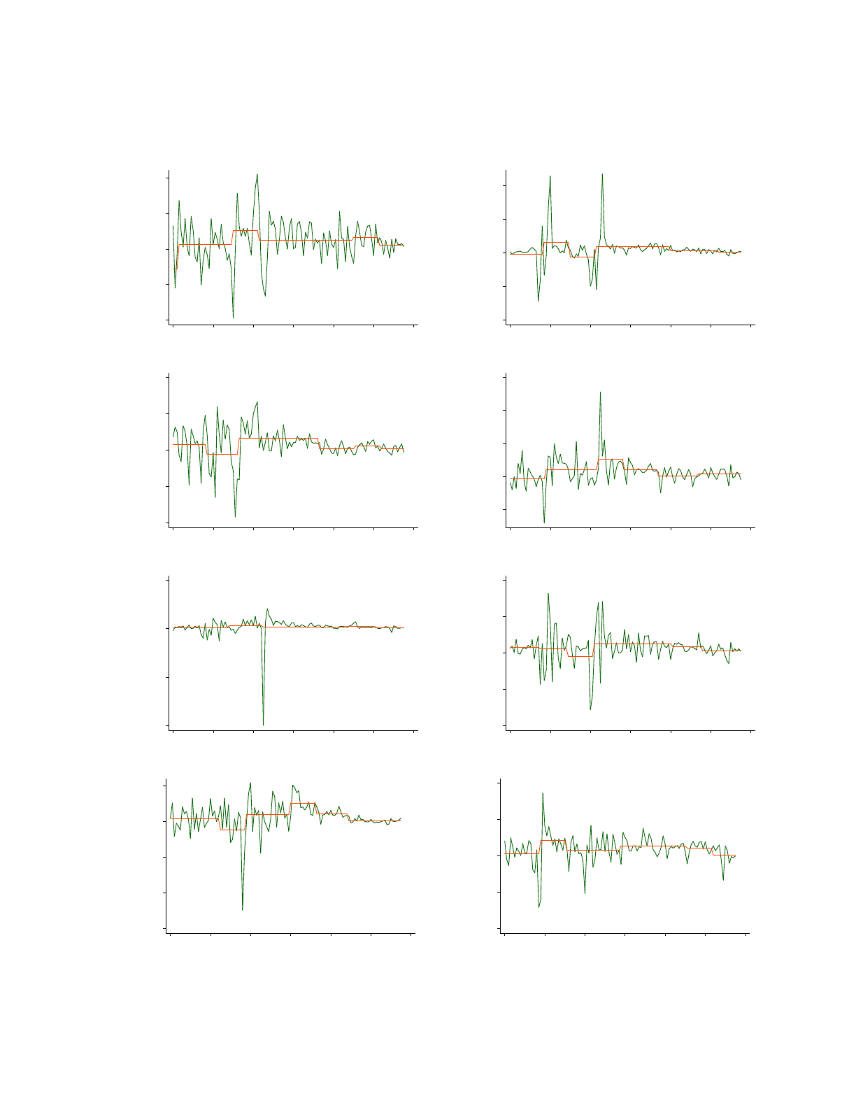
I.3. Structural break dates in TFP growth
-10 -5 0 5 10
1900 1920 1940 1960 1980 2000 2020
Year
TFP growth for AUS
-40 -20 0 20 40
1900 1920 1940 1960 1980 2000 2020
Year
TFP growth for BEL
-20 -10 0 10 20
1900 1920 1940 1960 1980 2000 2020
Year
TFP growth for CAN
-10 0 10 20 30
1900 1920 1940 1960 1980 2000 2020
Year
TFP growth for CHE
-100 -50 0 50
1900 1920 1940 1960 1980 2000 2020
Year
TFP growth for DEU
-20 -10 0 10 20
1900 1920 1940 1960 1980 2000 2020
Year
TFP growth for DNK
-30 -20 -10 0 10
1900 1920 1940 1960 1980 2000 2020
Year
TFP growth for ESP
-20 -10 0 10 20
1900 1920 1940 1960 1980 2000 2020
Year
TFP growth for FIN
A29

-40 -20 0 20 40
1900 1920 1940 1960 1980 2000 2020
Year
TFP growth for FRA
-10 -5 0 5
1900 1920 1940 1960 1980 2000 2020
Year
TFP growth for GBR
-20 -10 0 10 20 30
1900 1920 1940 1960 1980 2000 2020
Year
TFP growth for ITA
-80 -60 -40 -20 0 20
1900 1920 1940 1960 1980 2000 2020
Year
TFP growth for JPN
-40 -20 0 20 40 60
1900 1920 1940 1960 1980 2000 2020
Year
TFP growth for NLD
-10 -5 0 5 10 15
1900 1920 1940 1960 1980 2000 2020
Year
TFP growth for NOR
-10 -5 0 5 10 15
1900 1920 1940 1960 1980 2000 2020
Year
TFP growth for PRT
-10 -5 0 5 10 15
1900 1920 1940 1960 1980 2000 2020
Year
TFP growth for SWE
A30

-10 -5 0 5 10 15
1900 1920 1940 1960 1980 2000 2020
Year
TFP growth for USA
A31

Appendix references
Bergeaud, Antonin, Gilbert Cette, and R´emy Lecat. 2016. Productivity Trends in Advanced Countries
between 1890 and 2012. Review of Income and Wealth 62(3): 420–444.
Bernanke, Ben S., and Ilian Mihov. 1998. The Liquidity Effect and Long-run Neutrality. Carnegie-
Rochester Conference Series on Public Policy 49(1): 149–194.
Bhattarai, Saroj, Gauti B. Eggertsson, and Bulat Gafarov. Forthcoming. Time Consistency and
Duration of Government Debt: A Model of Quantitative Easing. Review of Economic Studies .
Bilbiie, Florin O. 2019. Optimal Forward Guidance. American Economic Journal: Macroeconomics
11(4): 310–45.
Bilbiie, Florin O. 2020. The New Keynesian cross. Journal of Monetary Economics 114: 90–108.
Blanchard, Olivier. 2016. Currency Wars, Coordination, and Capital Controls. NBER Working Paper
22388.
Calvo, Guillermo A. 1983. Staggered Prices in a Utility-maximizing Framework. Journal of Monetary
Economics 12(3): 383–398.
Driscoll, John C., and Aart C. Kraay. 1998. Consistent covariance matrix estimation with spatially
dependent panel data. Review of Economics and Statisticsfor 80(4): 549–560.
Durbin, J. 1959. Efficient Estimation of Parameters in Moving-Average Models. Biometrika 46(3/4):
306–316.
Fornaro, Luca, and Federica Romei. 2019. The Paradox of Global Thrift. American Economic Review
109(11): 3745–79.
Gourinchas, Pierre-Olivier. 2018. Monetary Policy Transmission in Emerging Markets: An Application
to Chile. In Monetary Policy and Global Spillovers: Mechanisms, Effects and Policy Measures,
edited by Enrique G. Mendoza, Ernesto Past´en, and Diego Saravia, volume 25 of Central Banking,
Analysis, and Economic Policies Book Series, chapter 8, 279–324. Santiago: Central Bank of Chile.
Imbs, Jean M. 1999. Technology, growth and the business cycle. Journal of Monetary Economics
44(1): 65–80.
Itskhoki, Oleg, and Dmitry Mukhin. 2021. Mussa Puzzle Redux. Working Paper 28950, National
Bureau of Economic Research.
Jiang, Zhengyang, Arvind Krishnamurthy, and Hanno Lustig. 2020. Dollar Safety and the Global
Financial Cycle. NBER Working Paper 27682.
Kuersteiner, Guido M. 2005. Automatic Inference For Infinite Order Vector Autoregressions. Econo-
metric Theory 21(1): 85–115.
Lewis, Richard, and Gregory C. Reinsel. 1985. Prediction of multivariate time series by autoregressive
model fitting. Journal of Multivariate Analysis 16(3): 393–411.
Lusompa, Amaze B. 2019. Local projections, autocorrelation, and efficiency. UC Irvine. Unpublished.
A32

Obstfeld, Maurice, and Kenneth Rogoff. 1995. Exchange rate dynamics redux. Journal of Political
Economy 103(3): 624–660.
Paul, Pascal. 2020. Historical patterns of inequality and productivity around financial crises. Federal
Reserve Bank of San Francisco Working Paper 2017-23.
Rey, H´el`ene. 2015. Dilemma not Trilemma: The Global Financial Cycle and Monetary Policy
Independence. NBER Working Paper 21162.
Wiener, Norbert, and Pesi Masani. 1958. The prediction theory of multivariate stochastic processes,
II: The linear predictor. Acta Mathematica 99(1): 93–137.
A33
