
CALMAC ID PGE0450
Pacific Gas and Electric Company
Energy Efficiency Program
Update of California Weather Files for Use in
Utility Energy Efficiency Programs and
Building Energy Standard Compliance Calculations
Publication Date March 6, 2020
Prepared by Joe Huang
White Box Technologies
346 Rheem Blvd., Suite 205A
Moraga CA 94556
Technical Editor Kati Pech
Pacific Gas and Electric Company
San Francisco, California
Project Managers Brian Arthur Smith
Pacific Gas and Electric Company
San Francisco, California
Richard S. Ridge
Ridge and Associates
San Rafael, California
LEGAL NOTICE
This report was prepared by Pacific Gas and Electric Company in collaboration with the California
Public Utilities Commission, the California Energy Commission, Southern California Edison Company,
San Diego Gas & Electric, and Southern California Gas Company. None of these entities nor any of its
employees and agents:
(1) make any written or oral warranty, expressed or implied, including, but not limited to those
concerning merchantability or fitness for a particular purpose;
(2) assume any legal liability or responsibility for the accuracy, completeness, or usefulness of any
information, apparatus, product, process, method, or policy contained herein; or represent that its
use would not infringe any privately-owned rights, including, but not limited to, patents, trademarks,
or copyrights.
2
Table of Contents
0.0
Executive Summary
3
1.0
PROJECT BACKGROUND
3
2.0
PROJECT OBJECTIVES
4
3.0
DATA
4
4.0
PROCESSING THE RAW DATA
8
5.0
PROGRAMS AND PROCEDURES
16
6.0
WEATHER FILE NAMES
21
7.0
WEATHER FILE FORMATS
21
8.0
SELECTION OF CALIFORNIA LOCATIONS
22
9.0
PRODUCTION OF CZ2018 AND CALEE2018 WEATHER FILES
26
10.0
RESULTS
32
11.0
CONCLUSIONS
41
12.0
RECOMMENDATIONS
41
13.0
REFERENCES
42
A.1
DESCRIPTION OF THE WEATHER FILES IN CSV FORMAT
44
3
Executive Summary
Accurate and up-to-date weather data is an essential component of building energy efficiency programs. It allows for
an objective assessment of energy savings from Energy Efficiency projects carried out by the utilities and provides a
firm technical basis for setting building energy efficiency goals for building energy standards and for verifying
compliance to the building energy standards.
For nearly a decade, the California Energy Commission (CEC) and the Investor-owned Utilities (IOUs) have relied
on the CZ2010 standard weather files for compliance calculations and normalizing energy savings from utility energy
programs. The increased public awareness that climate is an ever-changing dynamic system, coupled with perceptions
that California has been getting hotter in recent years, has spurred attention on updating the CZ2010 weather files to
correspond closer to current weather conditions.
The objectives of this project are to update the CZ2010 weather files with the most recent weather data resources,
including newly available satellite-derived solar radiation, and develop two customized versions of “typical year”
weather files. One version will be delivered to the CEC for use in developing the next version of the Title-24 Standards
and compliance calculations required by Title-24. The other version will be used by PG&E and other IOUs to support
their Energy Efficiency programs, including their use in building energy simulations and spreadsheet calculations to
determine energy savings from program activities and for normalizing that savings for weather variability. This project
will also provide IOU consultants and contractors with historical weather files over the last five years for the same
California locations to be covered by the “typical year” weather files. Such weather data are indispensable for
engineering assessment of actual building performance.
1. PROJECT BACKGROUND
Detailed and reliable weather data are critical to the California Energy Commission (CEC) for the maintenance and
enforcement of the Title 24 building standards and to the California Public Utilities Commission (CPUC) in the
assessment of Energy Efficiency (EE) programs being undertaken by the Investor-Owned Utilities (IOUs), although
the needs of the two institutions are somewhat different. The CEC needs a benchmark set of “typical year” weather
files to rationalize the energy efficiency level of the prescriptive option, which in turn establishes an energy budget
for the performance option that a building cannot exceed based on computer simulations done with the benchmark
weather files. Although there has been increased concern about future climate change, to date “typical year” weather
files are still constructed to replicate the most typical weather conditions of a past period of record, which was
originally 30 years but is now as short as 12 years to reflect more recent weather conditions. For almost 30 years,
starting from when Title-24 was first enacted in 1982, the CEC used the same set of 16 CTZ (California Thermal Zone)
weather files that were created by Crow (1983), and revised using the same data by Augustin (1991). The revised set
has been called the CTZXXRV2, where XX refers to the CTZ Climate Zone number.
A set of “typical year” weather files to replace the CTZXXRV2 files was finally created by White Box Technologies
(WBT) for the CEC in 2010. These are the CZ2010 weather files (Huang 2010), which will be in use until 2023 when
they in turn will be replaced by a set of weather files developed by the current project. Taking advantage of the
increased availability of raw weather data from NOAA’s Integrated Surface Database (ISD, Lott and Baldwin 2001),
as well as commercial satellite-derived solar radiation (CPR 2019), WBT was able to create CZ2010 files for 86
California locations extracted from 12 years of data from 1998 through 2009. Since the CEC had adopted the use of
TDVs (Time Dependent Valuations) as a metric for fuel prices, the CEC requested that the same “typical months”
be used for all 86 locations, because TDVs are dependent on utility district-wide demand, that in turn are dependent
on state-wide weather conditions,
The CPUC and IOUs need “typical year” weather data to control for interannual weather variations when estimating
savings for their energy efficiency programs in a two-step procedure. First, each EE program participant uses the
historical data from the most appropriate weather station so that the relationship between weather or temperature and
energy use can be more accurately estimated. Additionally, to estimate weather-normalized savings for these EE
programs, for the past eight years the IOUs have relied on the CZ2010 weather files. However, the use of the CZ2010s
to weather-normalize savings is increasingly suboptimal since (1) the CZ2010s do not reflect the typical weather
unique to each weather station but, as noted above, are based on the same typical months for all 86 locations, and (2)
the CZ2010s are based on weather conditions from 1998-2009, but California has experienced substantially warmer
summers in the eight years from 2010 through 2017.

4
Both the CEC and the IOUs recognize that temperatures over the last ten years have been among the hottest on record
and are expected to increase, and they have agreed that the CZ2010s need to be updated so that it can take these hotter
temperatures into account for both the CEC’s development of the next version of Title-24 and the CPUC’s and IOU’s
estimations of weather-normalized energy savings and building performance. In recognition of CEC’s needs for
supporting Title-24, this project has agreed to create this updated version of CZ2018
1
weather files in accordance to
the Commission’s preferences for using state-wide “typical months” and extending the period of record from 12 to 20
years (1998-2017). At the same time, for the IOUs, this represents an opportunity to create an alternate set of
CALEE2018 “typical year” weather files based on typical months unique to each location and keep the 12 year time
period (2006-2017) as used in the CZ2010s, thus improving the accuracy of their estimates of weather-normalized
savings over the next few years. This project report presents the research objectives of the CEC and the IOUs and
describes the methods and activities that have been carried out to achieve these objectives.
2. PROJECT OBJECTIVES
There are two sets of research objectives, one to satisfy the needs of stakeholders (e.g., the CPUC, IOUs, and
ratepayers) in the evaluation of EE programs in California and one to satisfy the needs of the CEC.
The research objectives for Energy Efficiency stakeholders are:
1. Update the CZ2010 reference files for each of the 86 Integrated Surface Database (ISD) weather stations in
California, plus 31 new additions, based on the most recent 12 calendar years of data for each station (2006-
2017). For convenience, these updated weather files for EE Evaluation will be referred in this report as the
CALEE2018 reference weather files.
2. Provide historical weather files of the last 5 years (2014-2018) for the same 117 weather stations as above.
The research objective for the California Energy Commission is:
Update the CZ2010 reference files for each of the 86 Integrated Surface Database (ISD) weather stations in
California, plus 11 new additions, for a total count of 97 locations, based on the most recent 20 calendar years of
data for each station (1998-2017). There are fewer locations than for the CALEE2018 files for two reasons: (1)
the use of statewide “typical months” meant that all stations had to have usable data for the same year, whereas
for the CALEE2018 files a station that lacks monthly data for a certain year would just skip that year in selecting
the “typical month”, (2) the longer 20 year period of record reduced the number of available locations. For
convenience, these updated weather files for Title-24 compliance calculations will be referred in this document
as the CZ2018 reference weather files.
3. DATA
All the raw weather data used in creating the roughly 2,300 weather files (117 locations x 20 years) came from two
sources: (1) the weather station data was obtained from the Integrated Surface Database (ISD) maintained by the
National Centers for Environmental Information (NCEI), which is a branch of the National Oceanic and Atmospheric
Administration (NOAA), (2) the satellite-derived solar radiation data was obtained from the National Solar Radiation
Database (NSRDB), maintained by the National Renewable Energy Laboratory in Golden, Colorado. Combining these
two sources of data has resulted in weather files of unprecedented reliability and accuracy, especially the solar
radiation data, which historically had been the most problematic climate parameter to obtain.
1
CZ2018 is the name given these by the PI and refers to the year the project was initiated. The CEC has indicated that they will
likely change the name to correspond to the next version of the Title-24 Standard for which the files will become the standard
weather data, possibly CZ2023.
5
3.1 The Integrated Surface Database (ISD)
The availability of raw weather data on the Internet has expanded tremendously over the past 15 years. In particular,
the US National Centers for Environmental Information (NCEI, formerly known before 2016 as the National Climatic
Data Center or NCDC) started in 2006 to make the ISD (Integrated Surface Database) available through the Web. The
ISD developed out of the NCDC’s role under a 1960’s World Meteorological Organization (WMO) resolution as the
world’s repository for surface observations, i.e., gathering and storing weather station reports from around the world.
For several decades these reports were stored on computer tapes, but starting in 1998, the NCDC (NCEI), in
partnership with the US Air Force and Navy, converted all the data to a common ASCII format and made them
accessible via the Web. Up until 2011, the ISD was free only for US government, academic, and non-profit
organizations, but since then it has been free for everyone. This database contains up to 40 years of weather data
contributed by over 35,000 weather stations around the world. Of this, the data for over 14,000 stations (roughly 2,600
US and 11,000 non-US) are of sufficient resolution and period-of-record for developing detailed hourly weather files.
Since the ISD is an archive of weather data reported by stations in the participating nations, the data should be the
same as that reported by the stations to their national meteorological bureaus. For the US stations in the ISD, they are
simply the weather reports contributed by various National Weather Service stations and can be regarded as the
standard for data completeness and reliability. A major benefit to the NCEI making the ISD database available on the
Web is that, in addition, the reporting format for the data has been unified. The ISD data are reported in a standard
DSI-3505 format containing 105 columns in fixed-field format for mandatory data elements, including Wind Speed
and Direction, Sky Condition, Visibility, Dry-bulb Temperature, Dew point Temperature, and Atmospheric Pressure,
followed by optional data elements in free-field format preceded by a three character alphanumeric code when reported
(NCDC 2003).
Although this DSI-3505 format may seem confusing and intimidating at first glance, its implementation by NCEI has
proven to be extremely consistent, and once the format has been correctly deciphered and the processing software
debugged, the PI has not experienced any problems due to the data format, a situation for which NCEI deserves more
recognition and acclaim.
For building energy simulations, the most useful optional data element was Cloud Cover, which is used by many solar
models to estimate solar radiation, but this element has become much less important with the advent of satellite-
derived solar radiation measurements, which are more complete, accurate, and easier to import into weather files.
Other optional data elements that potentially have use in building energy simulations are Liquid Precipitation (or
Rainfall) and Present Weather (for estimating rainfall or falling snow), while Visibility and Ceiling Height (reported
mainly for use in aviation) are considered mainly for consistency with other weather file formats, such as TMY2,
TMY3, or EPW. In addition to the observed data, these recent weather file formats also derive other climatic
parameters such as the Extraterrestrial Radiation, Illuminance, Aerosol Optical Depth, Surface Albedo, and
Precipitable Moisture.
It should be noted that the ISD is not a unified database, but an archive of weather data from around the world that
NCEI has converted to the same data format. As a result, the data quality within the ISD can vary tremendously. The
weather reports from major stations in the US, Canada, Europe, East Asia, etc., often have over 20,000 observations
per year, i.e., more than three observations every hour. On the other hand, smaller weather stations or stations in less
developed nations may provide too little weather data to create a usable weather file.
The data quality of the California weather stations in the ISD is comparatively good. Using 2017 as a benchmark year,
the ISD contained data for 174 California locations. Of these, 43 stations were discarded either because the files were
blank (2) or lacked Dry-bulb (4) or Dewpoint Temperature (35). The remaining 136 stations all report the four key
critical weather parameters of Dry-bulb and Dew point Temperature, Cloud Cover, and Wind Speed, although 14
stations had sizeable data gaps of up to one month during the year. Of the other 121 stations, 114 have complete hourly
records and require minimal processing, while one station reported data every six hours and six others reported data
only during working hours, i.e., from 9 am to 5 pm.
The PI has had over ten years of experience in processing raw ISD data files, combining them with satellite-derived
solar radiation data to create historical weather files, and then using the historical weather files to create “typical year”
6
weather files for various clients, including ASHRAE in producing the IWEC2 weather files (Huang 2011) and the
CEC in producing the CZ2010 weather files. These experiences have led the PI to adhere to two basic principles in
processing data into finished weather files.
The first principle is to never alter and clearly identify the raw data throughout the process, except for standard
conversions such as from standard pressure to station pressure, cloud cover in octets to tenths, and expanding the
liquid precipitation reported by duration (XX mm of rain per YY hours) to hourly values (see Section 4.1f for details).
There are many advantages with adhering to this principle: (1) when anomalous values appear, it’s easy to determine
whether the cause is the raw data or the data filling method, (2) when problems are identified in the data processing
or the processing methodology improved, these can often be amended in the processed file without having to go back
to the raw ISD data files.
The second principle is to fill all the missing data, especially for elements that are used in building energy simulation
programs. In the PI’s opinion, the key value of the processed climatic data is that it removes the need for the building
energy modeler to process the input weather data, with all the needed climatic information appearing in regular
sequence hour-by-hour. Although some may argue that "truth in advertising" requires that missing data elements be
shown as such, typically with a flag value such as "999", in most circumstances the creator of the weather files is
likely to have more experience in data filling. Additionally, the filled data are always clearly indicated so that users
can always override those values. In adherence to this principle, nearly all the climatic data elements in the finished
weather file are filled, especially those required by building energy simulation programs, including such stochastic
elements as Wind Direction, Cloud Cover, and Present Weather. Users of the weather files should be aware that such
filled values have limited reliability and that any analysis, such as calculating their frequency distribution or "wind
roses”, should be done only with the actual observed values. The only climatic data element for which data filling is
not attempted is Liquid Precipitation, or rainfall. Here, only the observed precipitation, after considerable processing,
is reported, with missing data assumed to signify no precipitation.
The following Section 4.1 describes the methodologies used in processing the observed climatic data elements, Section
4.2 describes the incorporation of satellite-derived solar radiation, and Section 4.3 covers the methodologies used in
calculating the other derived climatic data elements. Section 5 describes step-by-step the programs and procedures
that implement the described methodologies starting with the raw ISD data files and ending with the historical year
weather files. The selection of the "typical months" and the creation of the CZ2018 and CALEE2018 "typical year"
files from the historical weather files are described separately in Section 8 later in the report.
3.2 The National Solar Radiation Data Base (NSRDB)
Until the advent of weather satellites and the development of irradiance models to derive solar radiation from satellite
imagery, the solar radiation in standard weather files were all derived using analytical models for clear sky irradiance
and empirical models for all sky irradiance based in reported Cloud Cover and other climatic parameters. A good
summary of such modelling techniques can be found in Iqbal (1983). Although measured solar data might have been
used to calibrate the solar models, such data were too rare for direct use in weather files, and the use of solar models
was the only practical solution.
Since solar radiation was the only weather parameter that was calculated rather than directly measured, it was the most
contentious and challenging aspect in the creation of weather files. For example, the technical reports for the TMY2,
TMY3, IWEC, and IWEC2 weather sets all devoted the lengthiest discussion on deriving the solar radiation (Marion
and Urban 1995, Wilcox and Marion 2008, Thevenard and Brunger 2001, Huang. 2011).
There are numerous difficulties in modelling solar radiation due to limitations in both the models and the input data.
A review of Iqbal (1983) indicates that modelled solar radiation are generally reliable for the domain (location, time
of year, etc.) for which the model was developed but much less so when applied to other locations and times (Dutton
2006). Additionally, the key input value for cloud cover tends to be reported less regularly than temperature, humidity,
or wind, and the values are by human observation, which can be subjective.
The use of satellite imagery to calculate solar irradiance has many advantages. The data are comprehensive and
uninterrupted, now making solar irradiance the most readily available weather parameter of all. The technology for
7
deriving the incoming solar radiation at the surface from a satellite image of the cloud cover and reflected surface
radiation has been under development in several countries around the world for almost twenty years (see Perez et al.
2002 as an example).
Interest and governmental support for such work is largely derived from its clear benefits to the solar power industry,
where accurate estimates of solar resources affect site selection and economic evaluations. Starting in the early 2000’s,
commercial companies have provided satellite-derived solar and weather data to the solar industry, such as Clean
Power Research (CPR 2019) and Solargis (2019). Through collaborative agreements with governmental agencies or
financial institutions, these companies have made some of their data public, such as CPR’s SolarAnywhere portal
providing hourly solar for the US from 1998-2012 (CPR 2019b) or SolarGIS’s solar maps showing average annual
irradiance anywhere in the world (SolarGIS 2019b). However, their commercial data, e.g., hourly time-series of solar
irradiance, generally costs hundreds to over a thousand dollars per site per year. Starting in the early 2010’s, several
government-supported national or international agencies have also been established to provide satellite-derived solar
irradiance for different parts of the world for free or at a low price.
For the 2010 project to develop the CZ2010 weather files, the PI obtained satellite-derived solar radiation data
covering all of California from 1998 through 2009 that was purchased from CPR by the CEC and gained insights into
working with satellite-derived solar radiation. At the beginning of the current project, the PI had several discussions
with PG&E and the CEC about different options to obtain satellite-derived solar radiation data, with the consensus to
use the NSRDB instead.
The National Renewable Energy Laboratory (NREL) is a US Department of Energy laboratory that is recognized
throughout the world as a leading research center on solar energy. Since the 1990s, NREL has produced several
iterations of the National Solar Radiation Data Base (NSRDB) that contained 30 years of solar radiation and related
meteorological data. These were used to produce the TMY files that are the de-facto standard “typical year” weather
files for the US. Version 1 of the NSRDB NREL (1992) contained 1961-1990 data for 237 US locations, as did the
corollary TMY2 weather files (Marion and Urban 1995). Version 2 (Wilcox 2012) contained 1991-2010 data for 1,454
US locations, while the corollary TMY3 weather files contain 1,020 locations (Wilcox and Marion 2008).
Versions 1 and 2 were both based on standard weather station data (the same as recorded in the ISD) and have been
released online as sets of weather files. The hourly solar radiation was modeled using a cloud-based METSTAT model
(Marion and Urban 1995).
The current NSRDB is a major change from previous versions because it uses satellite-derived in place of modeled
solar radiation and the data is released through an interactive Web-based GIS application called the NSRDB Viewer
(NREL 2019a, Habte et al. 2017). The current version (v2.0.0) was developed using the Physical Solar Model (PSM)
using satellite imagery from 1998 through 2017. These images contain approximately “2 million 0.038-degree latitude
by 0.038-degree longitude surface pixels (nominally 4 km
2
)”, and the area covered “is bordered by longitudes 25° W
on the east and 175° W on the west, and by latitudes -20° S on the south and 65° N on the north” (NREL 2019b).
The NSRDB Viewer displays an interactive base map of the world with the areas covered by the NSRDB indicated
by isopleth maps of solar radiation (see Figure 1). The user can drag a pointer to a location and select the years, data
attributes, and download options, such as using UTC or local time, half hour or hour intervals, etc. Once the data are
ready, the user receives an e-mail with a download link.
Although the Viewer is handy for specifying and downloading a handful of solar files, since this project required
downloading nearly 3,000 station-years of solar data, the PI received help from NREL staff to use a Python API for
batch download of the solar data. Since NREL imposes limits on downloading to preserve bandwidth for other uses,
obtaining twenty years of solar data for 130 locations took about a week of time, and this had to be repeated at least
once within the past year as NREL upgraded from Version 2 to Version 3 of their Physical Solar Model (PSM V3.0.1)
(NREL 2019).

8
Figure 1. NSRDB Data Viewer Selection Screen
While the NSRDB Viewer also provides meteorological data, these are not from observations but from MERRA
reanalysis (Roth 2019) and should be regarded with caution. The Viewer can also provide “typical year” data extracted
from the time-series, but these should also be regarded with caution for the same reason. Lastly, it should be noted
that the solar irradiances are instantaneous values and not aggregated totals as needed for building energy simulations.
There is more discussion about this situation in Section 4.2.
4. PROCESSING THE RAW DATA
4.1 Processing ISD climatic data elements
The biggest challenge encountered in processing the observed climatic data is how to deal with missing data elements.
This project treats missing data elements in different ways depending on their importance and whether there are any
meaningful ways for interpolation. For those elements regarded as stochastic, such as wind direction and present
weather, the approach is to use a "step function" that repeats the last available data element for half of the duration
and repeats the next available data element for the remaining half of the duration of the missing interval. For those
elements regarded as sequential, such as pressure, wind speed, cloud cover, opaque cover, ceiling, and visibility, the
approach is to use linear interpolations. A more elaborate interpolation procedure has been developed for dry-bulb
and dew point temperatures, partly because of its importance in building energy simulations and partly because diurnal
temperature profiles are relatively predictable.
The reporting of liquid precipitation, i.e., rainfall, is rather distinct and requires special treatment. Although the
original intent was to simply pass on what was reported, i.e., multiple and often overlapping reports of rainfall amount
and duration, this is judged to be not very usable and frequently misleading to users. Hence, an attempt has been made
to interpret and reconcile the reported rainfall amounts and durations, that are then reported as simple hourly values.
For more information on the processing of liquid precipitation, see Section 4.1f.
a. Dry-Bulb and Dew Point Temperatures
To interpolate for missing dry-bulb temperatures, a two-step process has been used, with an optional third step added
to improve the nighttime temperature profile for the 4 or 5 stations that do not record temperatures at night.

9
In the first step of the two-step process, missing temperatures are filled using linear interpolation if the gap is less than
eight hours. If the gap is greater than eight hours, they are filled by repeating the temperatures at the same hours the
previous day, but with the beginning and end hours of the gap linearly interpolated to match the observed value. This
is done in the awk script ncdcfm7.awk described in Section 5.1b.
Figure 2 shows the application of this technique to repeat the last available daily profile while matching the beginning
and end temperatures of the gap, when there is a gap of two days in the data for Monterey Peninsula the week before
Christmas in 2017. The filled dry-bulb and dew point temperatures are shown by the dotted lines in blue for dry-bulb
and red for dew point temperatures.
Figure 2. Missing temperature data for Monterey WMO 724915 Dec. 16-26, 2017
In the second pass, the interpolated values for the hours from 6 to 19 are recalculated using the following Fourier
Series (Equation 1) based on the PI’s previous work with Q.Y. Zhang on Chinese weather data (Zhang et al. 2002):
θ(t) = b
0
+
{ b
n
cos( n
12
t) + a
n
sin (n
12
t) } (1)
where b
0
= 1/8
=
8
1k
θ(k)
b
n
= 1/4
=
8
1k
θ(k) cos
4
kn
a
n
= 1/4
=
8
1k
θ(k) sin
4
kn
n = nth term of the Fourier series
k = sequential number of temperature from hours 1 to 8 at three-hour intervals
θ(k) = k
th
observed temperature
t = local standard time
The main purpose for this rather elaborate procedure is to smooth the profile and capture the daily maximum occurring
during these hours for stations that do not have hourly data. Among the California stations, there is only one such
station, Eureka, which reports data every six hours, at the very bottom of data completeness for creating a weather file
(Figure 3). All the other California stations have close at least hourly reports, in which case this Fourier Series
technique is not needed. The Fourier interpolation is done in the fourier7.awk script, described more fully in Section
5.1
-10
-5
0
5
10
15
20
Temperature ( C )
December 16 - 26 , 2017
Dec 16 Dec 17 Dec 18 Dec 19 Dec 20 Dec 21 Dec 22 Dec 23 Dec 24 Dec 25 Dec 26

10
Figure 3. Dry-bulb and dew point temp in Eureka (WMO 725940) Feb. 23-28, 2017
The two-step procedure is applied to both the dry-bulb and dew point temperatures and appears to address two distinct
kinds of data gaps, the first being episodes when data are lost for an extended time, and the second being short regularly
repeating gaps within a day, e.g., when a station records data at three-hour intervals. However, there is a third type of
data gap that is not adequately addressed by the two-step procedure. There are four weather stations out of the 117 (El
Monte_747043, San-Clemente-Island-NAAS_722925, Torrance-Muni-AP_722955, and Whiteman-AP_745057) that
report weather conditions only during the day, but not at the night. With the two-step procedure, the results are straight
line interpolations from the early evening to the early morning hours, thus missing the nighttime minima typically
occurring between 3 and 5 a.m.
For these stations, a procedure has been developed that replaces the linearly interpolated values between the last
evening and the first morning hours, when the first morning temperature is lower than the last evening temperature,
and the interpolation period exceeds 8 hours, by a sine curve so that the nighttime minimum temperatures are also
captured.
θ(k) = cos (
24
)8*(2 +k
)*daily_range + daily_mean (2)
where θ = interpolated temperature
k = hour of day for temperature gap
daily_range = calculated from beginning and end temperatures of gap
daily_mean = calculated from beginning and end temperatures of gap
Although the procedure was developed for both dry-bulb and dew point temperatures, after testing the decision was
made to apply it only to the dry-bulb temperatures, and to use a simple linear interpolation for the dew point
temperatures. When the morning (dry-bulb) temperature is higher than the last available nighttime temperature, the
dry-bulb temperatures also revert to a simple linear interpolation, instead.
This optional third step is implemented with two brief awk scripts, dbtsine.awk and dptlinear.awk, and used to modify
the missing nighttime dry-bulb and dew point temperatures for these four stations. Figure 4 shows what happens when
this optional third step is applied to the Torrance station that did not report between Hours 19 and 5 on all days. The
dotted red line shows the linear interpolation from the two-step procedure, with straight lines during the missing hours,
while the solid red line shows the results from the sine curve to bring out the putative nighttime minima at Hour 5.
Figure 4. Dry-bulb and dew point temp for Torrance (WMO 722955) Sept. 5-11, 2017
-5
0
5
10
15
Temperature ( C )
February 23- 28 , 2017
10
15
20
25
30
Temperature (C )
Days starting September 5, 2017
Feb 23 Feb 24 Feb 25 Feb 26 Feb 27 Feb 28
Feb 23 Feb 24
Sept 5 Sept 6 Sept 7 Sept 8 Sept 9 Sept 10 Sept 11

11
When there are stations in close proximity, spatial interpolation was also used with good results. The top plot in Figure
5 shows that in 2011 San Jose Reid Airport was missing dry-bulb temperatures shown in blue line from July 12 to 26,
and from July 28 to August 19, with the two periods indicated by the light grey tint. However, San Jose Mineta Airport
had complete temperature records throughout those two periods, as indicated by the red line. The two airports are
located within six miles of each other in similar suburban settings, although Reid is twice as far away from the south
end of San Francisco Bay and at a slightly higher elevation. Comparing their temperatures in the periods when both
were reporting data, it’s clear that then temperatures are virtually identical, except for the daytime maxima where Reid
consistently showed temperatures that were 2-3° C higher.
Figure 5. Temperatures at San Jose Reid and Mineta Airports in July and August 2011
A script was written to track the differences in temperature by time of day and the daily temperature range, since it’s
apparent that differences in daily maxima was reduced on cool and cloudy days. This script was then used to spatially
interpolate the temperatures at Reid Airport during the two data gap periods (see lower plot of Figure 5).
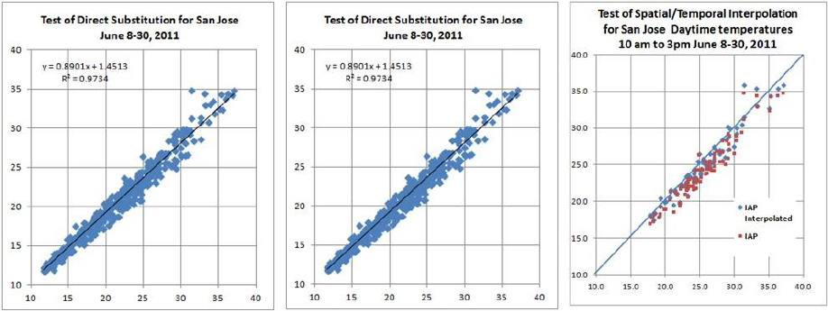
To test the accuracy of this spatial interpolation, it was also applied to the period immediately before the data gaps
and the interpolated temperatures compared to the actual temperatures at Reid Airport (see top plot of Figure 6). The
X-Y plots (see bottom plot of Figure 6 on the next page) comparing the actual to the interpolated temperature by direct
substitution (left) and spatial-temporal interpolation (center) show that the latter has a slightly higher R
2
. Since the
temperature differences only appear around the noontime peak, the third X-Y plot on the right compares direct
substitution (red dots) to spatial interpolation (blue dots) only for hours between 10 am and 3 pm. This shows that
spatial-temporal interpolation is clearly better than direct substitution with a standard deviation of less than 1° C.
Figure 6. Comparison of direct substitution to spatial-temporal interpolation using San Jose Mineta
Airport to fill in missing temperature data in San Jose Reid Airport, summer 2011.
12
This spatial-temporal procedure was applied in several other cases where there were extended time gaps in temperature
records.
b. Pressure
The ISD reports standard pressure that has been corrected to sea level. These are calculated back to the actual station
pressure using the following equation (Sandhurst 2009):
Station Pressure = Sea Level Pressure * e - elev / (temp * 29.263) (3)
where Station Pressure = barometric pressure in millibars (hectopascals)
Sea Level Pressure = reported pressure at sea level in millibars (hectopascals)
elev = station elevation in meters
temp = current temperature in Kelvin (K)
Many of the weather files have no or very infrequent recordings of standard pressure. If pressure data are regularly
recorded, linear interpolation is used for missing values. If pressure data are infrequent or nonexistent, values from a
suitable nearby station with values are substituted. If no suitable station can be found, a constant mean sea level
pressure of 1013.25 millibars (29.92 in Hg) is used. This data element is processed by the awk script ncdcfm7.awk.
c. Wind Speed
To interpolate for missing wind speed data, linear approximations are used. This data element is processed in the awk
script ncdcfm7.awk.
d. Wind Direction
To fill in missing wind direction data, a "step function" is used whereby the last observed wind direction is repeated
for the first half of the missing hours, and the next observed wind direction is repeated for the second half of the
missing hours. These filled wind directions have scant reliability, since there is no credible method to estimate wind
direction in the absence of data, and should not be used in any analysis, such as calculating the frequency distribution
of wind directions or "wind roses", which should be done only with the actual observed values. This data element is
processed in the awk script ncdcfm7.awk.
e. Cloud Cover
The ISD data format contains fields for Total Sky Cover and Opaque Sky Cover, but the latter are mostly missing.
The Total Sky Cover is read as octets and converted to tenths of Cloud Cover. To interpolate for missing Cloud Cover
data, linear approximations are used. Since the Opaque Sky Cover is not used in any building energy simulation
program and mostly missing in the ISD, this climatic element is one of the few that has been left as "99", a flag to
13
indicate missing data. This data element is processed in the awk script ncdcfm7.awk. Sky Cover records are much less
important in this project because of the use of satellite-derived solar.
f. Liquid Precipitation
Liquid Precipitation or rainfall has been included in the TMY3 format for the first time. For building energy
simulations, this data element is needed for simulating the performance of green roofs. Unfortunately, the way that
rainfall is reported in the ISD is difficult to interpret. There are two fields giving the amount of rainfall in mm and the
time period in hours covered by the recording. For example, a recording may indicate there are 20 mm (0.79 in.) of
rainfall over the past 12 hours. The difficulty arises when there are multiple recordings for overlapping time periods
that may be inconsistent, as when the 24-hour rainfall exceeds the sum of the reported rainfall for the day, or even
contradictory, as when the 24-hour rainfall is less than that reported for a shorter period within that day. To reconcile
these reports, an algorithm has been developed to convert them to hourly rainfall using the following assumptions:
1)
forward marching, i.e., never adjust any previous reported value;
2)
if a report is multi-hour, distribute rainfall equally for the preceding number of hours reported;
3)
if reports are overlapping, subtract the amounts already reported, and apportion the remaining rainfall
equally to the hours following the previous report;
4)
for reports that are completely overlapping, i.e., multiple reports (this happens most often with a 24-
hour report overlaying 6-hour reports), if the overlapping report is less than the sum of already reported
amounts, ignore; if more, distribute the unaccounted rainfall equally to hours that are unreported; but
if there are no unreported hours, ignore the excess;
5)
if duration is unreported (99), assume duration is from last report, unless it's over 24 hours in which
case assume 24 hours.
This algorithm was first developed by the PI for the ASHRAE IWEC2 weather files and has been tested on over 6,000
ISD files from around the world, including several hundred in the US and Canada. That testing shows that: (a) while
only 5.6% of the international stations reported no rainfall (333 out of 5988), 26.8% of the US and Canadian stations
did so (425 out of 1585), suggesting that a significant number of North American may be failing to report rainfall at
all; (b) the reported rainfall for many station fluctuated greatly depending on the year; and (c) a few locations reported
impossibly high rainfall that can be an order of magnitude greater than their reported annual average.
Continued review of the derived liquid precipitation for all 3,012 IWEC2 weather files showed that a small number
of isolated reports of excessive rainfall were skewing the total annual precipitation in a quarter of the files. For
example, in 263 files a single report of hourly precipitation above 50 mm/hr (spread out over several hours due to the
distribution algorithm) made up more than half of the total annual precipitation. To weed out such unusual and possibly
spurious liquid precipitation reports, two cutoff limits were added to exclude hourly precipitation values above 50
mm/hour or daily precipitation values above 150 mm/day.
For more discussion of this algorithm and why the cutoff limits were instituted, please refer to Huang et al. 2011, pp.
56-45. This data element is also processed in the awk script ncdcfm7.awk, to which this algorithm has been
incorporated.
g. Present Weather
Present Weather refers to a numerical code by meteorologists to indicate the weather condition, e.g., rain, driving rain,
snow, sleet, fog, etc. Although NREL included a 10-digit code for Present Weather in the TMY2 format (Marion and
Urban 1995), NREL eliminated Present Weather in their later TMY3 format (Wilcox and Marion 2008). Because of
its usefulness for indicating instances of rain or snow fall, the PI extracted the Present Weather code that appears in
the ISD and inserted it as an additional field at the end of the TMY3 format. However, the Present Weather code in
the ISD is the internationally recognized METAR 2-digit code for rather than the obsolete 10-digit code used in the
TMY2 (NCDC 2003). This Present Weather code appears in the CSV and FIN4 formats of the weather files, but not
in the EPW or BINM formats. To fill in missing Present Weather data, a "step function" is used whereby the last

14
observed present weather is repeated for the first half of the missing hours, and the next observed present weather is
repeated for the second half of the missing hours. This data element is also processed in the awk script ncdcfm7.awk.
4.2 Processing satellite-derived solar from the NSRDB
Importing satellite-derived solar radiation data into a standard weather file can be as simple as a line-by-line insertion
or substitution of original modelled radiation, provided that the nomenclature and time conventions are consistent
between the two sets of data. Unfortunately, often they are not, making it important to check and make any necessary
adjustments to the solar data.
The problem lies with synchronizing the solar data time with that of the weather files. The difficulty of time
synchronization is complicated because there are two ways that solar radiation is reported, either as an instantaneous
rate or as a total integrated over the time step. In the US, solar radiation on a weather file is the aggregated total over
the previous time step. For example, Hour 12 would show the total amount of solar radiation from 11:00 to 12:00.
This is also the format needed for building energy simulation programs. However, in most other countries and in
satellite-derived solar databases (including the NSRDB), it is the instantaneous rate at the time step, e.g., Hour 12
would show the rate of solar radiation at 12:00. Since the vast majority of weather files are hourly, the units are the
same between both types of data, i.e., 1 watt-hour == 1 W/hr, so the only difference arises from half-hour time data.
Since the NSRDB provides satellite-derived solar values at the half-hour, a simple way to convert NSRDB solar values
to the US convention would be to calculate the hourly solar as
0.25*SOL
-1hr
+0.50*SOL
-30min
+0.25*SOL
hr
. (4)
Although a 30-minute discrepancy in the solar radiation might seem like a minor difference, it can cause numerous
strange effects, especially at sunrise and sunset hours, since the energy simulation program would be computing sun
positions that would be off by half an hour.
For years, the PI tried with moderate success various methods to detect synchronization problems, such as counting
the number of hours with non-zero sun angles and no solar radiation, i.e., the sun is above the horizon but there is no
solar radiation, etc. In 2018, the author learned of a graphical method that proved to be very useful by plotting the
ratio between the global and extraterrestrial horizontal irradiance (Kt/Et) against the ratio between the diffuse and
global horizontal irradiance (Kd/Kt). Figure 7 shows the striking difference in the plots when the solar radiation is
synchronized (middle) compare to when they’re ahead (left) or behind (right) by a half hour. The thick red line shows
the theoretical relationship as calculated by the well-known Erbs Model (Erbs, Klein, and Duffy 1982).
Figure 7. Kd/Kt versus Kt/Et for Devil’s Island WI 2016 with the
time stamp for solar irradiance at various shifts
0.0
0.2
0.4
0.6
0.8
1.0
0.0 0.2 0.4 0.6 0.8 1.0
Kd/Kt
Kt/Et
Solar irradiance shifted -00:30 hour
0.0
0.2
0.4
0.6
0.8
1.0
0.0 0.2 0.4 0.6 0.8 1.0
Kd/Kt
Kt/Et
Solar Irradiance unshifted
0.0
0.2
0.4
0.6
0.8
1.0
0.0 0.2 0.4 0.6 0.8 1.0
Kd/Kt
Kt/Et
Solar Irradiance shifted +00:30

15
Use of this graphical technique has assured the PI that the possibility of faulty time synchronization of the solar
radiation no longer exists.
During the production of the CZ2018 and CALEE2018 files, the PI noticed a sharp morning spike in the solar radiation
during the summer months in more than 30 locations, all situated along or near the Pacific coast. The top plot on
Figure 8 shows the average daily solar profile by month for Arcata. NREL staff considered the satellite imagery of
cloud conditions at sunrise too unreliable due to the very low sun angles, and so the imagery was ignored, and the
cloud cover was assumed to be clear. Since there is a high frequency of morning fog along the coast during the summer,
this would be detected in the satellite imagery for the second or third hour after sunrise, thus causing the pronounced
spikes in the solar hourly profile from May through August. Until NREL decides to modify its model assumptions, a
simple correction has been added so that the cosine of the solar angle (Kt*cos(Z)) is the same for hours during the
spike and immediately after the spike. The lower plot of Figure 8 shows the average monthly solar profiles after the
correction has been added.
Figure 8. Average daily solar profile by month for Arcata
4.3 Calculating other derived climatic data elements
a. Illuminance
The total horizontal, diffuse horizontal, and direct normal illuminances in lux and the zenith illuminance in cd/m
2
are
calculated using a luminance efficacy model developed by Perez et al. (1990). The inputs to the model are the global
horizontal and direct normal irradiance, solar zenith angle, and the dew point temperature. It is not clear if these
illuminances are used in any building energy simulation program.
b. Albedo and Aerosol Optical Depth
These derived values appear in the TMY3 weather file format, probably because they are needed as inputs for the
Metstat Model used by NREL to derive solar radiation (NREL 1995). The albedo shown in the TMY3 files refers to
the geographical region of the station, not the immediate surroundings for the building (which is of more interest to
building energy simulations), and is a monthly value obtained from the Earth Radiation Budget Experiment (ERBE)
satellite data base available for a 1º by 1º grid (Wilcox 2009). The Optical Aerosol Depth is also a derived value, the
calculation for which is described cursorily in NREL 1995. Since neither of these two values is used for the solar
modeling, nor have relevance for building energy simulations, they have not been calculated and a “9900” code
inserted in the weather files to indicate missing data.
GHI
DNI
16
5. PROGRAMS AND PROCEDURES
5.1 Main procedure for processing weather files
The processing of the historical year weather files is done using a series of awk scripts and a Fortran program, that are
called by a MS-DOS batch file mkncdc3.bat (see Figure 9 for listing). When mkncdc3 is called, it requires 11
arguments in sequential order giving (1) output subdirectory name, (2) year, (3) station name, (4) first station (WMO)
number, (5) second station number, (6) WMO region, (7) time zone, (8) time zone code, (9) latitude, (10) longitude,
(11) elevation (m), and (12) Köppen climate region designation. Figure 10 shows an excerpt from the main
mkallncdc.bat file invoking a series of test runs repeated for various purposes.
Figure 9. Listing of the mkncdc3.bat batch file
rem ONE-STEP PROCEDURE FOR GENERATING HISTORICAL WEATHER FILES FROM ISH DATA
rem by Joe Huang Dec. 11, 2005
rem modified Aug 28, 2006 for processing all ISH data files
rem modified Feb 18, 2009 for ASHRAE project
rem modified May 11, 2009 to work with doewthm, fmtwth2m, and wthfmt2m
rem preliminary clean-up if old files exist
erase *.TMP
erase OUT*.*
erase WEATHR.TMP
rem set paths
set ISH=C:\HomeHDJoe\Duplicate\SU_Fenxian_HDD
rem set OutDir=J:\HomeHDJoe\Duplicate\NewLaptopJoe\Wthdat\NCDC\%1
set OutDir=%1
set/a thisyear=%2
set stanam=%3
set filenam=%3"_"%4
rem Step 0: truncate ISH file to needed data, read prev. or following year's files for missing hours
rem and convert to local time
rem
rem erase STATS.OUT
erase %3%thisyr%.DAT
erase %4-%5-*
set/a thisyr=%thisyear%-2000
if %thisyr% LSS 0 set/a thisyr=%thisyr%+100
if %thisyr% LSS 10 set thisyr=0%thisyr%
set timezone=%7
set/a lastyear=%thisyear%-1
gunzip < %ISH%\%lastyear%\%4-%5-%lastyear%.gz > scratch.tmp
tail -n 24 scratch.tmp > RAWDATA.TMP
erase scratch.tmp
gunzip < %ISH%\%thisyear%\%4-%5-%thisyear%.gz >> RAWDATA.TMP
pause
set/a nextyear=%thisyear%+1
gunzip < %ISH%\%nextyear%\%4-%5-%nextyear%.gz > scratch.tmp
head -n 24 scratch.tmp >> RAWDATA.TMP
erase scratch.tmp
awk2001 -f UTIL\readfil6.awk staname=%filenam% station=%4 yr=%thisyear% timezone=%7 RAWDATA.TMP
copy OUT.DAT %filenam%_%thisyr%.DAT
rem copy STATS.OUT %filenam%_%thisyr%.STAT
rem ..\..\UTIL\zip -j %OutDir%\%3DAT.ZIP %filenam%_%thisyr%.DAT
Rem zip -j %OutDir%\%3DAT.ZIP %filenam%_%thisyr%.DAT
Rem erase RAWDATA.TMP
Rem erase %filenam%_%thisyr%.DAT
rem erase STATS.OUT
rem Step 1: get *.DAT file from ZIP file and process to fill in missing values by linear interpolation
rem input = [location][year].DAT, output = OUT.TMP
shift
shift
shift
awk2006 -f UTIL\ncdcfm7.awk loc=%stanam% yr=%thisyear% wmo=%3 tz=%4 tzcode=%5 lat=%6 lon=%7 elev=%8 koeppen=%9 OUT.DAT
rem ..\..\UTIL\zip -j %OutDir%\%32DAT.ZIP %filenam%_%thisyr%.2DAT
rem erase OUT.DAT
rem Step 2: modify weather file with fourier interpolation for temperatures, and make wyec2 format weather file
rem (don't do this - fourier4.awk has formatting problems, fourier5 has logic problems, i.e., overwrites good data YJH 06_0828)
rem input = OUT.TMP, outputs = OUT2.DAT, WEATHR.TMP (full file in WYEC2 format without solar data)
awk -f UTIL\fourier7.awk OUT.TMP > OUT2.DAT
rem disable until solved YJH 09)0618
rem copy OUT.TMP OUT2.DAT
rem Step 3: use doewthm2 to calculate solar and pack weather into DOE *.BINM
rem inputs = WEATHR.TMP (OUT2.DAT), INPUT.TMP, HEADER.TMP (both created by fix0.awk from stninfo4.txt)
rem outputs = NEWTH.TMP (DOE-2 binary file), OUT3.DAT (fin file), IWEC.TMP (TMY2 format file)
if exist WEATHR.TMP erase WEATHR.TMP
awk -f UTIL\fix0.awk year=%thisyear% OUT2.DAT
rem copy OUT2.DAT %OutDir%\%filenam%"_"%thisyr%.OUT2 >nul
copy OUT2.DAT WEATHR.TMP

17
c:\wthdat\UTIL\doewthm2
Rem if exist %OutDir%\%filenam%"_"%thisyr%.BINM erase %OutDir%\%filenam%"_"%thisyr%.BINM
Rem copy NEWTH.TMP %OutDir%\%filenam%"_"%thisyr%.BINM >nul
Rem if exist %OutDir%\%filenam%"_"%thisyr%.IW2 erase %OutDir%\%filenam%"_"%thisyr%.IW2
rem killed for ISHRAE2 runs sed 's/ //' IWEC.TMP > %OutDir%\%filenam%"_"%thisyr%.IW2
Rem if exist %OutDir%\%filenam%"_"%thisyr%.FIN3 erase %OutDir%\%filenam%"_"%thisyr%.FIN3
copy OUT3.DAT %OutDir%\%filenam%"_"%thisyr%.FIN3
erase OUTPUT.
rem Step 4: clean up any left over files, and zip all saved files to [Location][year].ZIP file
erase OUT3.DAT
erase *.TMP
erase WEATHER.*
erase FMTWTH.INP
erase SOLAR.TMP
erase %OutDir%\%filenam%"_"%thisyr%.ZIP
Rem ..\..\UTIL\zip -j %OutDir%\%stanam%DOE2.ZIP %OutDir%\%filenam%"_"%thisyr%.BINM
Rem ..\..\UTIL\zip -j %OutDir%\%stanam%DOE2.ZIP %OutDir%\%filenam%"_"%thisyr%.STA
Rem ..\..\UTIL\zip -j %OutDir%\%stanam%FIN.ZIP %OutDir%\%filenam%"_"%thisyr%.FIN2
Rem erase %OutDir%\%filenam%"_"%thisyr%.BINM
Rem erase %OutDir%\%filenam%"_"%thisyr%.STA
Rem erase %OutDir%\%filenam%"_"%thisyr%.FIN2
Figure 10. Excerpt of mkallncdc.bat master batch file
@rem call mkncdc6 ISH2017\USA 2017 CA_BISHOP-AP 724800 23157 4 -8.0 NAP 37.371 -118.358 1250 Csb 0.97
@rem call mkncdc6 ISH2017\USA 2017 CA_MERCED-CASTLE-AFB 724810 23203 4 -8.0 NAP 37.383 -120.567 58 BSk 0.90
@rem call mkncdc6 ISH2017\USA 2017 CA_MERCED-MUNI-MACREADY 724815 23257 4 -8.0 NAP 37.285 -120.513 46 BSk 0.87
@rem call mkncdc6 ISH2017\USA 2017 CA_VACAVILLE-NUT-TREE 724828 93241 4 -8.0 NAP 38.378 -121.958 33 Csa 1.09
call mkncdc6 ISH2017\USA 2017 CA_SACRAMENTO-EXECUTIVE-AP 724830 23232 4 -8.0 NAP 38.507 -121.495 4 Csa 1.06
@rem call mkncdc6 ISH2017\USA 2017 CA_SACRAMENTO-MATHER-FL 724833 23206 4 -8.0 NAP 38.567 -121.300 30 Csa 1.11
@rem call mkncdc6 ISH2017\USA 2017 CA_MCCLELLAN-AFB 724836 23208 4 -8.0 NAP 38.667 -121.400 23 Csa
@rem call mkncdc6 ISH2017\USA 2017 CA_BEALE-AFB 724837 93216 4 -8.0 NAP 39.133 -121.433 34 Csa 1.11
@rem call mkncdc6 ISH2017\USA 2017 CA_YUBA-CO 724838 93205 4 -8.0 NAP 39.102 -121.568 18 Csa 1.07
@rem call mkncdc6 ISH2017\USA 2017 CA_SACRAMENTO-METRO-AP 724839 93225 4 -8.0 NAP 38.696 -121.590 7 Csa 1.06
@rem call mkncdc6 ISH2017\USA 2017 NV_NORTH-LAS-VEGAS 724846 53123 4 -8.0 NAP 36.212 -115.196 671 BWk 1.01
@rem call mkncdc6 ISH2017\USA 2017 CA_MONTEREY-PENINSULA 724915 23259 4 -8.0 NAP 36.588 -121.845 50 Csb 1.08
@rem call mkncdc6 ISH2017\USA 2017 CA_STOCKTON-METRO-AP 724920 23237 4 -8.0 NAP 37.889 -121.226 7 Csa 1.03
@rem call mkncdc6 ISH2017\USA 2017 CA_MODESTO-CITY-CO-AP 724926 23258 4 -8.0 NAP 37.624 -120.951 22 Csa 1.05
@rem call mkncdc6 ISH2017\USA 2017 CA_LIVERMORE-MUNI-AP 724927 23285 4 -8.0 NAP 37.693 -121.814 119 Csb 1.00
@rem call mkncdc6 ISH2017\USA 2017 CA_OAKLAND-METRO-AP 724930 23230 4 -8.0 NAP 37.721 -122.221 1 Csb 1.09
@rem call mkncdc6 ISH2017\USA 2017 CA_PALO-ALTO-AP 724937 23289 4 -8.0 NAP 37.467 -122.117 2 Csb 1.05
@rem call mkncdc6 ISH2017\USA 2017 CA_SAN-CARLOS-AP 724938 93231 4 -8.0 NAP 37.517 -122.250 1 Csb 1.05
@rem call mkncdc6 ISH2017\USA 2017 CA_SAN-FRANCISCO-IAP 724940 23234 4 -8.0 NAP 37.620 -122.365 2 Csb 1.11
@rem call mkncdc6 ISH2017\USA 2017 CA_SAN-JOSE-IAP 724945 23293 4 -8.0 NAP 37.359 -121.924 15 Csb 1.06
@rem call mkncdc6 ISH2017\USA 2017 CA_SAN-JOSE-REID-HILLV 724946 93232 4 -8.0 NAP 37.333 -121.817 40 Csb 1.04
Figure 11 is a simplified flow chart showing the steps invoked by mkncdc3.bat to go from the raw ISD data files at
the top to the completed historical year weather file in three formats at the bottom.
2
The "main path" shown on the left
part of Figure 11 are the procedural steps used to process all the weather files. The items shown on the right with
dashed lines indicate additional steps there were used to process a small percentage of the weather files.
The following descriptions of the awk scripts or Fortran program used in the main path shown in Figure 11 explains
briefly their functions and capabilities.
5.1a readfil6.awk is an awk script the deciphers the raw ISD file, converts from GMT to local time, and prints out
the climatic parameters of interest in a new file. Since the ISD files are stored in GMT, readfil6.awk also reads the
last 24 records from the previous year and the first 24 records of the following year in order to capture the entire year
in local time, as well as to allow data filling for missing hours at the beginning and end of each year. Figure 12 shows
the first 24 lines of the intermediate file for Sacramento Executive Airport 2017 generated by readfil6 from reading
the raw ISD file. The data are essentially unchanged but put in a more readable form with blanks as separators, and
the time stamp has been changed from GMT to local standard time.
2
This batch script does not include the insertion of the satellite-derived solar radiation, nor does it include the selection of the
“typical months” and creation of the final CZ2018 or CALEE2018 “typical year” weather files. That is a different procedure which
will be described later in Section 6).

18
Figure 11. Flow chart of processing ISD weather files
.
out2.dat
(clean hourly file of
observed data elements)
readfil6.awk
(extracts data of interest,
converts to local time)
ISD raw data file
out3.dat
(fixed field format
with derived solar)
weather.binm
(modified DOE-2
binary format)
doewthm2
(calculates derived values
for solar radiation,
illuminance, etc., outputs
three types of files )
IWEC.out
(TMY3 CSV format)
dbtsine.awk
(sine curve interpolation
of dry-bulb temps)
dptlinear.awk
(linear interpolation
of dewpoint temps)
Optional step for stations with
no nighttime data
(input can be either
out2.dat or out3.dat)
ncdcfm7.awk
(fills/interpolates missing data
fourier7.awk
(Fourier interpolation of
temps)
out.dat
(data file in local time)
Limited hand editing of bogus
data in very small number of
files
mergeisdsatsol
(merges satellite-derive
Solar radiation onto
out3.dat file)
*.epw
(EPW format)
EnergyPlus weather
(converts CSV file to
epw format)

19
Figure 12. Sample intermediate format file produced by readfil6.awk
for Sacramento Executive Airport WMO 724830 - first 24 records of 2017
724830 201612312353 +0050 +0033 10136 0026 140 99 99 99 016093 22000 9999 999 1 01000095
724830 201701010053 +0056 +0044 10135 0046 140 99 99 99 016093 22000 9999 999 1 01000095
724830 201701010059 +9999 +9999 99999 9999 999 99 99 99 999999 99999 9999 999 1 24000395
724830 201701010153 +0067 +0050 10132 0051 140 99 99 99 016093 00549 9999 999 1 01000095
724830 201701010253 +0067 +0050 10142 0031 150 99 99 99 016093 00549 9999 999 1 01000095
724830 201701010353 +0061 +0050 10136 0041 140 99 99 99 016093 00671 9999 999 2 01000095 2400039
724830 201701010453 +0061 +0044 10127 0036 140 99 99 99 016093 00732 9999 999 1 01000095
724830 201701010553 +0061 +0050 10132 0031 150 99 99 99 016093 00792 9999 999 1 01000095
724830 201701010653 +0061 +0050 10137 0031 140 99 99 99 016093 00853 9999 999 1 01000095
724830 201701010753 +0061 +0050 10138 0026 150 99 99 99 016093 00792 9999 999 1 01000095
724830 201701010853 +0061 +0044 10136 0036 160 99 99 99 016093 00792 9999 999 1 01000095
724830 201701010944 +0067 +0050 99999 0046 150 99 99 99 016093 00945 9999 999 0
724830 201701010951 +0070 +0050 99999 0041 150 99 99 99 016093 00762 9999 999 0
724830 201701010953 +0067 +0050 10143 0041 150 99 99 99 016093 00762 9999 999 1 01000095
724830 201701011017 +0072 +0044 99999 0036 160 99 99 99 016093 00914 9999 999 0
724830 201701011051 +0070 +0050 99999 0036 150 99 99 99 016093 00792 9999 999 0
724830 201701011053 +0072 +0050 10143 0026 160 99 99 99 016093 01006 9999 999 1 01000095
724830 201701011116 +0072 +0050 99999 0031 170 99 99 99 016093 00762 9999 999 0
724830 201701011153 +0083 +0056 10137 0026 999 99 99 99 016093 00762 9999 999 1 01000095
724830 201701011200 +0083 +0056 99999 0041 190 99 99 99 016093 01036 9999 999 0
724830 201701011210 +0083 +0056 99999 0021 210 99 99 99 016093 00488 9999 999 0
724830 201701011253 +0089 +0056 10128 0036 190 99 99 99 016093 00549 9999 999 1 01000095
724830 201701011353 +0094 +0056 10124 0036 190 99 99 99 016093 00762 9999 999 1 01000095
724830 201701011401 +0094 +0056 99999 0031 200 99 99 99 016093 00945 9999 999 0
5.1b ncdcfm7.awk is the main awk script with over 900 lines that reads the intermediate output file from
readfil6.awk, and processes all the observed climatic data elements by filling in the missing data, throwing out
redundant or sub-hourly data, and adding single-letter flags to each interpolated element. The methodologies for
interpolating missing data elements are described previously in Section 4.1. The algorithms used in ncdcfm7.awk to
process the different climatic data elements are all similar, apart from that for liquid precipitation or rainfall. For the
other elements, ncdcfm7.awk keeps track of the last available value, the interpolation period, and the current value.
Depending on the data filling method chosen for that element, ncdcfm7.awk calculates the interpolated value for each
missing hour and stores it in an array, along with a single-letter flag appended directly after the value. To illustrate the
general method for data-filling, Figure 13 shows how ncdcfm7.awk handles wind speed, one of the simplest elements
to process.
Figure 13. Excerpt from ncdcfm7.awk for processing wind speed
# WIND SPEED
if (wspd !~/9999/)
{
wspd = wspd/10
if (lastwspd == 999) lastwspd = wspd
wspdinter = hrofyr - lastwspdtime
wspdrecords = int(hrofyr) - int(lastwspdtime)
if (wspdrecords > 0)
for (i=1;i<=wspdrecords;i++)
{
residual = i + int(lastwspdtime)-lastwspdtime
iwspd = lastwspd + (wspd - lastwspd)*(residual/wspdinter)
itime = lastwspdtime + residual
if (itime > 0 && itime <= tothrs )
{
xwspdinter[int(itime)]=wspdinter
xwspdrecords[int(itime)]=wspdrecords
xiwspd[int(itime)]=iwspd
}
if (itime > 0 && itime <= tothrs )
{
if (i < wspdrecords)
xwspdflag[int(itime)]="L"
else
xwspdflag[int(itime)]=" "
}
}
lastwspd= wspd
lastwspdtime = hrofyr
}
The output from ncdcfm7.awk is another intermediate text file of standard length (either 8760 hours or 8784 hours for
leap years) with all climatic parameters filled in, but no solar radiation data. The format of this intermediate text file

20
is identical to that of the OUT2.DAT and OUT3.DAT files mentioned in the next two steps, which only refine the
filled temperature values and add the derived solar. It should be pointed out that ncdcfm7.awk and doewth2 form the
core of the weather processing method first developed by the PI in 2006, and which has been continually refined and
used in all subsequent projects to create weather files.
5.1c. fourier7.awk is an awk script that reads the intermediate output from ncdcfm7.awk and replaces any linearly
interpolated dry-bulb and dew point temperature between the hours of 6 and 19 with a Fourier Series. The output file
is called OUT2.DAT and contains all the information of the final weather file, except for the solar radiation. Figure
14 shows a sample OUT2.DAT file for Sacramento Executive Airport corresponding to the intermediate data shown
in Figure 12. Because the raw data is so complete, the only interpolated values in Figure 14 are those for Hour 16 or
4:00 pm. The interpolated values are identified by a single appended letter, L for linear interpolation, F for Fourier
interpolation, R for repeat of the last available value, and X for missing value.
Figure 14. Sample OUT2.DAT file produced by ncdcfm7.awk and fourier7.awk for Sacramento
Executive Airport WMO 724830 January 1, 2017
CA_SACRAMENTO-EXECUTIVE-AP 724830 38.507 -121.495 4 4 -8.0 NAP Csa
DBT DPT Press Altim Sky Opq WSpd Wnd TotSol DirNorm Pres
Year Mo Dy Hr (C) (C) (mb) (inHg) Cov (m/s) Dir (W/m2) (W/m2) Wth Rain Visib Ceil
2017 1 1 1 5.7 4.5 1013.0 5R 99R 4.7 140 05R 0R 16093 22000
2017 1 1 2 6.7 5.0 1012.8 5R 99R 4.9 140 05R 0R 16093 549
2017 1 1 3 6.6 5.0 1013.6 5R 99R 3.2 150 05R 0F 16093 563
2017 1 1 4 6.1 4.9 1013.0 5R 99R 4.0 140 05R 0R 16093 678
2017 1 1 5 6.1 4.5 1012.3 5R 99R 3.5 140 05R 0R 16093 739
2017 1 1 6 6.1 5.0 1012.8 5R 99R 3.1 150 05R 0R 16093 799
2017 1 1 7 6.1 5.0 1013.2 5R 99R 3.0 140 05R 0R 16093 845
2017 1 1 8 6.1 4.9 1013.3 5R 99R 2.7 150 05R 0R 16093 792
2017 1 1 9 6.2 4.5 1013.2 5R 99R 3.7 160 05R 0R 16093 813
2017 1 1 10 6.8 4.8 1013.8 5R 99R 4.0 150 05R 0R 16093 806
2017 1 1 11 7.2 5.0 1013.7 5R 99R 2.8 160 05R 0R 16093 931
2017 1 1 12 8.3 5.6 1013.1 5R 99R 4.1 190 05R 0R 16093 1036
2017 1 1 13 9.0 5.6 1012.3 5R 99R 3.6 190 05R 0R 16093 573
2017 1 1 14 9.4 5.6 1011.9 5 99R 3.2 200 05R 0R 16093 922
2017 1 1 15 9.9 5.4 1011.5 4 99R 3.5 180 05R 0N 16093 22000
2017 1 1 16 9.4L 3.8L 1011.3L 0L 99R 3.0L 200R 05R 0R 16093L 22000R
2017 1 1 17 9.1 3.3 1011.3 0 99R 2.5 160 05R 0R 16093 22000
2017 1 1 18 9.0 2.7 1011.3 0L 99R 2.2 160 05R 0R 16093 22000
2017 1 1 19 9.2 1.8 1011.5 0 99R 3.0 190 05R 0R 16093 2134
2017 1 1 20 7.7 2.9 1011.7 0L 99R 2.8 180 05R 0R 16093 22000
2017 1 1 21 7.1 3.3 1012.5 0L 99R 4.0 200 05R 0R 16093 2303
2017 1 1 22 6.7 3.3 1013.1 0L 99R 3.8 190 05R 0R 16093 2438
2017 1 1 23 6.7 3.3 1013.9 0L 99R 4.9 220 05R 0F 16093 2438
2017 1 1 24 6.6 3.2 1013.9 0 99R 3.4 200 05R 0F 16093 2438
5.1d. doewthm2 is a heavily modified version of the DOE-2 weather processor, which is written in Fortran 77. It
reads the OUT2.DAT file from the previous step, and derives the total global horizontal, direct normal, and diffuse
horizontal solar radiation using the Zhang-Huang Model (Zhang, Huang, and Lang 2002), as well as the other derived
climatic elements of extraterrestrial solar radiation (total horizontal and direct normal), illuminance (global horizontal,
direct, and diffuse), and zenith luminance. If satellite-derived solar radiation is available, these modeled solar radiation
values are replaced, and doewthm2 is rerun to calculate the illuminances and produce the other two output files
mentioned below.
doewthm2 produces three outputs files: (1) OUT3.DAT in the same text format as in OUT2.DAT (referred to by the
project team as *.FIN4 (meaning “final”) format, (2) IWEC.OUT, another text file in the TMY3 CSV format and (3)
WEATHER.BINM, a binary format that is an enhanced version of DOE-2’s *.BIN packed weather file format.
3
Figure
15 shows the final OUT3.DAT appearance for the same Sacramento Executive Airport 2017 file shown in Figure 14
where the modeled solar has been replaced by the satellite-derived solar radiation.
3
The BINM format was developed by the PI for the ASHRAE IWEC2 project. It is an extension of the BIN format used by DOE-
2. To reduce file size, the BIN format records temperatures in integer F, pressures in inches of mercury to one decimal point, and
solar radiation in integer BTU/ft
2
-hr. The BINM format increases the precision of the following climate variables by one significant
place: dry-bulb temperature, wet bulb temperature, pressure, total solar radiation, and direct normal solar. To maintain backwards
compatibility, this was done by adding additional integers at the end of each record.
21
Figure 15. Sample OUT3.DAT file produced by doewthm2
for Sacramento Executive Airport 24830 January 1, 2017
(same format as OUT2.DAT with satellite-derived solar radiation)
CA_SACRAMENTO-EXECUTIVE-AP 724830S 38.507 -121.495 4 4 -8.0 NAP Csa
DBT DPT Press Altim Sky Opq WSpd Wnd SatGHI SatDNI Pres
Year Mo Dy Hr (C) (C) (mb) (inHg) Cov Cov (m/s) Dir (W/m2) (W/m2) Wth Rain Visib Ceil SolarZ
2017 1 1 1 5.7 4.5 1013.0 5R 99R 4.7 140 0.0 0.0 5R 0R 16093 22000 0.0000
2017 1 1 2 6.7 5.0 1012.8 5R 99R 4.9 140 0.0 0.0 5R 0R 16093 549 0.0000
2017 1 1 3 6.6 5.0 1013.6 5R 99R 3.2 150 0.0 0.0 5R 0F 16093 563 0.0000
2017 1 1 4 6.1 4.9 1013.0 5R 99R 4.0 140 0.0 0.0 5R 0R 16093 678 0.0000
2017 1 1 5 6.1 4.5 1012.3 5R 99R 3.5 140 0.0 0.0 5R 0R 16093 739 0.0000
2017 1 1 6 6.1 5.0 1012.8 5R 99R 3.1 150 0.0 0.0 5R 0R 16093 799 0.0000
2017 1 1 7 6.1 5.0 1013.2 5R 99R 3.0 140 0.0 0.0 5R 0R 16093 845 0.0000
2017 1 1 8 6.1 4.9 1013.3 5R 99R 2.7 150 15.0 66.0 5R 0R 16093 792 0.0243
2017 1 1 9 6.2 4.5 1013.2 5R 99R 3.7 160 136.0 442.0 5R 0R 16093 813 0.1696
2017 1 1 10 6.8 4.8 1013.8 5R 99R 4.0 150 86.5 148.5 5R 0R 16093 806 0.3059
2017 1 1 11 7.2 5.0 1013.7 5R 99R 2.8 160 59.8 0.0 5R 0R 16093 931 0.4057
2017 1 1 12 8.3 5.6 1013.1 5R 99R 4.1 190 224.3 114.0 5R 0R 16093 1036 0.4616
2017 1 1 13 9.0 5.6 1012.3 5R 99R 3.6 190 148.0 13.0 5R 0R 16093 573 0.4696
2017 1 1 14 9.4 5.6 1011.9 5 99R 3.2 200 109.0 0.0 5R 0R 16093 922 0.4293
2017 1 1 15 9.9 5.4 1011.5 4 99R 3.5 180 131.8 160.8 5R 0N 16093 22000 0.3433
2017 1 1 16 9.6F 4.3F 1011.3L 0L 99R 3.0L 200R 185.5 541.3 5R 0R 16093L 22000R 0.2179
2017 1 1 17 9.1 3.3 1011.3 0 99R 2.5 160 46.3 204.5 5R 0R 16093 22000 0.0697
2017 1 1 18 9.0 2.7 1011.3 0L 99R 2.2 160 0.0 0.0 5R 0R 16093 22000 0.0000
2017 1 1 19 9.2 1.8 1011.5 0 99R 3.0 190 0.0 0.0 5R 0R 16093 2134 0.0000
2017 1 1 20 7.7 2.9 1011.7 0L 99R 2.8 180 0.0 0.0 5R 0R 16093 22000 0.0000
2017 1 1 21 7.1 3.3 1012.5 0L 99R 4.0 200 0.0 0.0 5R 0R 16093 2303 0.0000
2017 1 1 22 6.7 3.3 1013.1 0L 99R 3.8 190 0.0 0.0 5R 0R 16093 2438 0.0000
2017 1 1 23 6.7 3.3 1013.9 0L 99R 4.9 220 0.0 0.0 5R 0F 16093 2438 0.0000
2017 1 1 24 6.6 3.2 1013.9 0 99R 3.4 200 0.0 0.0 5R 0F 16093 2438 0.0000
6. WEATHER FILE NAMES
The ISD, as well as many previous weather data sets, e.g., IWEC and TMY3, used only station WMO numbers as
their file names. For example, 724830-23232-2017 is the ISD file for Sacramento Executive Airport, 037760.IW2 is
the IWEC file for London Gatwick, and 725033TY.CSV is the TMY3 file for New York Central Park. The weather
file names in this project follows previous efforts by the PI to combine legibility with precision. The file names use
two underscores ("_") to separate the two-letter state abbreviation adopted by the US Postal Service in 1963 from the
location name, the station’s WMO number, and finally the last two digits of the year or the name of the “typical year”
set, e.g., CZ2018 or CALEE2018. All blank spaces and special characters in the location name are replaced by hyphens,
and a period (“.”) is used only once as the separator to the file extension. For example, the name of the 2017
Sacramento Executive Airport file is CA_SACRAMENTO-EXECUTIVE-AIRPORT_724830_17.[extension]. The
extension refers to the format of the file, i.e., *.FIN4, *.CSV, *.epw, or *.BINM.
7. WEATHER FILE FORMATS
The archival versions of the weather files are all in the *.FIN4 format, which the PI prefers because it’s a fixed-field
format that’s easy to read in any text editor, with self-describing column headings and data flags. Line 1 contains the
header information on the weather station: Station Name, WMO Station Number, Latitude (N+, S-), Longitude (E+,
W-), Elevation (m), WMO region number, Time Zone, ISO-3166 3-letter Country Code, and Köppen climate
classification. Lines 2 and 3 contain the column headings, from left to right: Year, Month, Day, Hour, Dry-bulb
Temperature (C), Dew Point Temperature (C), Pressure (mb), Sky Cover (tenths), Opaque Cover (tenths), Wind Speed
(m/s), Wind Direction (degrees), Global Horizontal (W/m
2
), Direct Normal (W/m
2
), Present Weather, Rainfall
(0.1mm), Visibility (m), Ceiling Height (m), and SolarZ. For all the recorded parameters, i.e., everything but the solar
radiation, there are optional single capital letter flags to indicate that the value is interpolated (L = linear, F = Fourier
Series, R = repeat last available value, etc.). The column widths can be found in this following Fortran write statement:
WRITE(IOUT3,5001) KYR,IM,KDOM,KHR,XDB,DBFLAG,XDP, (5)
. DPFLAG,XPRESS,PRSFLAG,KCOV,COVFLAG,KOPQ,OPQFLAG,XWNDSP,
. WSPDFLAG,KWNDIR,WDIRFLAG,KSOL,KDN,IPRSWTH,PWTHFLAG,
. KRAIN,RAINFLAG,IVISIB,VISBFLAG,ICEIL,CEILFLAG,COSZAV
5001 FORMAT(I4,1X,I2,1X,I2,1X,I2,1X,F5.1,A1,1X,F6.1,A1,1X,F6.1,
. A1,8X,I2,A1,1X,I2,A1,1X,F4.1,A1,1X,I3,A1,1X,F6.1,
. 2X,F6.1,1X,I3,A1,1X,I4,A1,1X,I6,A1,1X,I6,A1,1X,F6.4)

22
There is an Excel template file to import a *.FIN4 file into Excel that correctly parses the data columns between values
and the flags available at http://www.whiteboxtechnologies.com/UTIL/Fin4toExcel.xlsm. Users who prefer a TMY3-
compatible CSV format can obtain them from White Box Technologies by e-mailing
support@whiteboxtechnologies.com. This CSV format is described in the Appendix to this report.
For general users, the weather files have been written into *.epw and *.BINM formats and uploaded to the
http://www.calmac.org/weather.asp website for public download. The *.epw format was developed for the EnergyPlus
program, but it can also be read by some other programs. Information on the *.epw format can be found in the
documentation for EnergyPlus. The *.BINM format is compatible with the *.BIN format developed for the DOE-2
program. The *.BIN and *.BINM are binary file formats that are not directly readable, but there are programs such as
Elements (https://bigladdersoftware.com/projects/elements/downloads.html) that can convert files to readable txt.
8. SELECTION OF CALIFORNIA LOCATIONS
The period of record and the completeness of the climatic data elements are used as criteria to determine whether a
station has enough data for creating an CALEE2018 or CZ2018 weather file. The overall periods of record considered
for all stations are the 12 years from 2006 to 2017 for CALEE2018 and the 20 years from 1998 to 2017 for CZ2018.
Out of that period of record, a station must have at least seven years of usable data, defined as those years with an
average of at least 4 recordings per day for dry-bulb and dew point temperatures, cloud cover, and wind speed.
Furthermore, to insure uniformity in the recordings over time, each month must have at least 124 recordings.
A total of 117 weather stations were found to meet these criteria. When the ISD data are inspected in more detail, the
stations are found to fall into three distinct types: A) those with hourly or sub-hourly data, B) those with hourly data
only during daytime hours, or C) those with data every six hours. Of the 117 weather stations, 107 fall in the “A”
category, 9 fall in the “B” category, and only one falls in the “C” category.
Figure 16 is a sketch map of California showing the location of all 117 weather stations. Table 1 lists the 117 stations
with their header information (station name, WMO number, latitude, longitude, and elevation) as well as the metadata
on their data class (A, B, or C), number of available years, and average number of observations per day for the three
key parameters of dry-bulb temperature, dew point temperature, and wind speed. The statistics file also has metadata
on cloud cover, but since the files use satellite-derived solar radiation, the metadata on cloud cover are ignored. Since
91% of the weather files have full hourly data, and 90% of these have the complete record of years (12 for CALEE2018
and 20 for CZ2018), the raw data should be considered very complete, with the exception of some anomalies for a
few stations and years.

23
Figure 16. Locations for CALEE2018 and CZ2018 weather files

24
Table 1. List of CALEE2018 and CZ2018 weather files
City
Station name WMO Lat (N) Lon (W)
Elev
(m)
Data
Class
No.
Years
No.
obs/day
Data
Class
No.
Years
No.
obs/day
Alturas ALTURAS 725958 41.483 120.567 1330 A 12 23.0 A 20 23.6
Arcata-AP ARCATA-AP 725945 40.978 124.109 64 A 12 22.7 A 20 23.5
Auburn-Muni-AP AUBURN-MUNI-AP 720267 38.955 121.082 466 A 12 22.4 A 13 23.1
Bakersfield-Meadows-Field BAKERSFIELD-MEADOWS-FLD 723840 35.434 119.054 149 A 12 23.5 A 20 24.5
Bishop-AP BISHOP-AP 724800 37.373 118.363 1263 A 12 23.4 A 20 23.7
Blue-Canyon-AP BLUE-CANYON-AP 725845 39.292 120.708 1610 A 12 22.6 A 20 23.5
Blythe-Riverside-Co-AP BLYTHE-RIVERSIDE-CO-AP 747188 33.619 114.717 119 A 12 22.7 A 20 23.8
Burbank-Glendale-Pasadena-AP BURBANK-GLNDLE-PASAD-AP 722880 34.201 118.359 223 A 12 22.4 A 17 23.4
Camarillo-AP CAMARILLO(AWOS) 723926 34.217 119.083 23 A 12 22.8 A 20 23.8
Camp-Pendleton-MCAS CAMP-PENDLETON-MCAS 722926 33.300 117.350 23 A 12 21.4 A 20 22.7
Carlsbad-Mcclellan CARLSBAD-MCCLELLAN 722927 33.128 117.279 100 A 12 22.6 A 20 23.6
Chico-Muni-AP CHICO-MUNI-AP 724973 39.795 121.858 72 A 9 21.0
China-Lake-NAF CHINA-LAKE-NAF 746120 35.683 117.683 695 A 12 22.1 A 20 19.3
Chino-AP CHINO-AIRPORT 722899 33.975 117.636 207 A 12 22.4 A 20 23.5
Concord-Buchanan-Field BUCHANAN-FIELD-AP 724950 37.992 122.055 5 A 12 22.7 A 20 23.5
Corona-Muni-AP CORONA-MUNI-ARPT 720333 33.900 117.600 163 A 12 21.8
Crescent-City-Faa-AP CRESCENT-CITY-FAA-AP 725946 41.780 124.237 16 A 12 22.9 A 18 23.7
Daggett-Barstow-AP DAGGETT-BARSTOW-DAGGETT-AP 723815 34.854 116.787 588 A 12 22.4 A 20 23.5
Davis-AP DAVIS 720576 38.533 121.783 21 A 8 22.0
El-Centro-NAF EL-CENTRO-NAF 722810 32.817 115.683 -12 A 12 22.4 A 20 19.4
Eureka EUREKA 725940 40.800 124.150 18 C 12 3.8 C 20 3.8
Fairfield-Travis-AF TRAVIS-FLD-AFB 745160 38.267 121.933 18 A 12 22.6 A 18 23.6
Fresno-Yosemite-IAP FRESNO-YOSEMITE-IAP 723890 36.780 119.719 101 A 12 23.6 A 20 24.6
Fullerton-Muni-AP FULLERTON-MUNI-AP 722976 33.872 117.979 29 A 12 22.6 A 20 23.6
Half-Moon-Bay-AP HALF-MOON-BAY-AIRPOR 720646 37.517 122.500 20 A 8 21.6
Hanford-Muni-AP HANFORD-MUNI-AP 723898 36.319 119.629 75 A 12 22.4 A 18 23.2
Hawthorne-Jack-Northrop-Field JACK-NORTHROP-FLD-H 722956 33.917 118.333 20 A 12 22.7 A 20 23.6
Hayward-AP HAYWARD-EXECUTIVE-AI 725850 37.650 122.117 19 A 12 22.6 A 20 23.5
Hollister-Muni HOLLISTER-MUNI 749179 36.900 121.417 72 A 9 22.6
Imperial-Beach-Ream-Field IMPERIAL-BEACH-REAM-FLD 722909 32.567 117.117 7 A 12 20.9 B 20 18.6
Imperial IMPERIAL 747185 32.834 115.579 -17 A 12 22.7 A 20 23.6
Kern-Co-Edwards-AFB EDWARDS-AFB 723810 34.933 117.900 705 A 12 21.6 A 20 21.6
Kings-Co-Lemoore-Reeves-NAS LEMOORE-REEVES-NAS 747020 36.333 119.950 71 A 12 21.6 A 20 20.8
Lincoln-Rgnl LINCOLN-RGNL 720614 38.909 121.351 37 A 8 22.4
Lake-Tahoe LAKE-TAHOE 725847 38.894 119.995 1912 A 12 22.5 A 20 23.3
Lancaster-Wm-Fox-Field LANCASTER-GEN-WM-FOX-FIELD 723816 34.741 118.219 712 A 12 22.9 A 20 23.8
Livermore-Muni-AP LIVERMORE-MUNI-AP 724927 37.694 121.817 121 A 12 22.5 A 20 23.6
Lompoc LOMPOC(AWOS) 722895 34.666 120.467 26 A 12 20.5 A 20 20.4
Long-Beach-Daugherty-Field LONG-BEACH-DAUGHERTY-FLD 722970 33.828 118.163 12 A 12 23.5 A 20 24.5
Los-Alamitos-AAF LOS-ALAMITOS-AAF 722975 33.790 118.052 10 A 12 20.9 B 18 18.9
Los-Angeles-Downtown-USC LOS-ANGELES-DOWNTOWN-USC 722874 34.028 118.296 56 A 12 22.4 A 18 23.5
Los-Angeles-IAP LOS-ANGELES-INTL-AP 722950 33.938 118.406 99 A 12 23.5 A 18 24.6
Los-Angeles-Whiteman-AP WHITEMAN-AP 745057 34.259 118.413 305 B 8 9.6
Madera-Muni-AP MADERA-MUNI 745046 36.988 120.111 77 A 12 21.9 A 18 22.9
Mammoth-Yosemite MAMMOTH-YOSEMITE 723894 37.457 118.838 2172 A 12 20.9 B 20 15.8
Marysville-Beale-AFB BEALE-AFB 724837 39.136 121.436 34 A 12 22.0 A 18 19.3
Merced-Castle-AFB MERCED-CASTLE-AFB 724810 37.383 120.567 58 A 11 19.8
Merced-MacReady-Field MERCED-MACREADY-FLD 724815 37.285 120.514 48 A 12 22.6 A 20 23.2
Modesto-City-Co-AP MODESTO-CITY-CO-AP 724926 37.624 120.951 22 A 12 22.5 A 20 23.4
Mojave MOJAVE 722953 35.059 118.152 850 B 11 17.4
Montague-Siskiyou-Co-AP MONTAGUE-SISKIYOU-CO-AP 725955 41.781 122.468 805 A 12 22.6 A 20 23.4
Monterey-Peninsula MONTEREY-PENINSULA 724915 36.588 121.845 67 A 12 22.7 A 18 23.6
Mount-Shasta MOUNT-SHASTA 725957 41.333 122.333 1077 A 12 22.9 A 18 23.7
Mountain-View-Moffett-Field MOUNTAIN-VIEW-MOFFETT-FLD 745090 37.415 122.048 10 A 12 22.9 A 13 23.6
Napa-Co NAPA-CO 724955 38.213 122.280 17 A 12 22.7 A 20 23.6
Needles-AP NEEDLES-AP 723805 34.766 114.623 278 A 12 22.7 A 20 23.9
Novato-Gnoss-Field-AP GNOSS-FIELD-AIRPORT 720406 38.150 122.550 1 A 11 21.9
Oakland-Metro-AP OAKLAND-METRO-AP 724930 37.755 122.221 26 A 12 22.6 A 18 23.7
Oceanside-Muni-AP OCEANSIDE-MUNI-AP 722934 33.219 117.349 8 A 12 22.7 A 18 23.3
Ontario-IAP ONTARIO-INTL-AP 747040 34.050 117.567 287 A 12 22.6 A 17 23.5
CALEE2018
CZ2018

25
Table 1. List of CALEE2018 and CZ2018 weather files (cont.)
City
Station name WMO Lat (N) Lon (W)
Elev
(m)
Data
Class
No.
Years
No.
obs/day
Data
Class
No.
Years
No.
obs/day
Oroville OROVILLE 745048 39.490 121.618 58 A 12 22.6 A 18 23.0
Oxnard-AP OXNARD-AP 723927 34.201 119.206 20 A 12 22.6 A 20 23.5
Palm-Springs-IAP PALM-SPRINGS-INTL 722868 33.828 116.505 137 A 12 22.4 A 20 23.6
Palm-Springs-Thermal-AP PALM-SPRINGS-THERMAL-AP 747187 33.628 116.160 -36 A 12 22.7 A 20 23.6
Palmdale-AP PALMDALE-AP 723820 34.629 118.084 787 A 12 22.4 A 20 23.5
Palo-Alto-AP PALO-ALTO-AIRPORT 724937 37.461 122.115 1 B 12 12.7 B 20 14.1
Paso-Robles-Muni-AP PASO-ROBLES-MUNICIPAL-AP 723965 35.673 120.627 249 A 12 22.7 A 20 23.6
Placerville-AP PLACERVILLE-AIRPORT 720645 38.717 120.750 787 A 8 22.6
Point-Mugu-Nf POINT-MUGU-NF 723910 34.117 119.117 3 A 12 21.9 A 20 20.8
Porterville PORTERVILLE(AWOS) 723895 36.033 119.067 135 A 12 22.6 A 20 23.3
Ramona RAMONA 745056 33.033 116.917 424 A 12 22.5 A 18 23.4
Red-Bluff-Muni-AP RED-BLUFF-MUNICIPAL-AP 725910 40.152 122.254 107 A 12 23.5 A 20 24.4
Redding-Muni-AP REDDING-MUNICIPAL-AP 725920 40.515 122.313 153 A 12 23.4 A 20 24.4
Riverside-March-AFB RIVERSIDE-MARCH-AFB 722860 33.881 117.259 467 A 12 22.9 A 20 23.6
Riverside-Muni-AP RIVERSIDE-MUNI 722869 33.952 117.439 253 A 12 22.6 A 20 23.3
Sacramento-Executive-AP SACRAMENTO-EXECUTIVE-AP 724830 38.513 121.493 7 A 12 22.4 A 20 23.5
Sacramento-Mather-Field SACRAMENTO-MATHER-FL 724833 38.554 121.285 29 A 12 18.7 A 17 19.3
Sacramento-McClellan-AFB MCCLELLAN-AFB 724836 38.667 121.400 23 A 7 22.4
Sacramento-Metro-AP SACRAMENTO-METRO-AP 724839 38.696 121.590 10 A 12 22.6 A 20 23.4
Salinas-Muni-AP SALINAS-MUNI 725930 36.650 121.600 24 A 12 22.4 A 19 23.6
San-Carlos-AP SAN-CARLOS-AP 724938 37.512 122.249 1 A 12 19.2 B 20 17.1
San-Clemente-Is-NAAS SAN-CLEMENTE-IS-NAAS 722925 33.023 118.588 55 B 12 8.2 B 20 9.3
San-Clemente-San-Mateo-Point SAN-MATEO-POINT 722928 33.286 117.456 27 A 8 20.4
San-Diego-Brown-Fld-Muni-AP BROWN-FLD-MUNI 722904 32.572 116.979 157 A 12 22.5 A 18 23.6
San-Diego-Gillespie SAN-DIEGO-GILLESPIE 722907 32.826 116.973 118 B 12 11.6 B 15 13.0
San-Diego-IAP SAN-DIEGO-LINDBERGH-FIELD 722900 32.735 117.169 8 A 12 23.6 A 20 24.6
San-Diego-Miramar-MCAS MIRAMAR-MCAS 722931 32.867 117.150 146 A 12 22.8 A 15 23.3
San-Diego-Montgomery SAN-DIEGO-MONTGOMER 722903 32.816 117.139 128 A 12 22.6 A 20 23.6
San-Diego-N-Island-NAS SAN-DIEGO-NORTH-ISLAND-NAS 722906 32.700 117.200 7 A 12 22.4 A 20 23.1
San-Francisco-IAP SAN-FRANCISCO-IAP 724940 37.620 122.398 5 A 12 23.6 A 20 24.5
San-Jose-IAP SAN-JOSE-INTL-AP 724945 37.362 121.928 15 A 12 22.6 A 20 23.5
San-Jose-Reid-Hillview SAN-JOSE-REID-HILLV 724946 37.333 121.820 40 B 12 13.0 B 20 15.0
San-Luis-Co-Rgnl-AP SAN-LUIS-CO-RGNL 722897 35.237 120.641 63 A 12 22.7 A 20 23.7
San-Nicholas-Island SAN-NICHOLAS-ISLAND 722910 33.240 119.458 153 B 12 11.5 B 20 14.1
Sandberg SANDBERG 723830 34.744 118.724 1378 A 12 23.3 A 18 23.8
Santa-Ana-AP SANTA-ANA-JOHN-WAYNE-AP 722977 33.680 117.866 16 A 12 22.5 A 20 23.5
Santa-Barbara-Muni-AP SANTA-BARBARA-MUNICIPAL-AP 723925 34.426 119.844 6 A 12 22.5 A 14 23.6
Santa-Catalina-Catalina-AP SANTA-CATALINA-CATALINA-AP 722920 33.405 118.416 488 A 12 22.6 A 20 23.4
Santa-Maria-Public-AP SANTA-MARIA-PUBLIC-AP 723940 34.916 120.465 72 A 12 23.4 A 20 24.5
Santa-Monica-Muni-AP SANTA-MONICA-MUNI 722885 34.016 118.451 53 A 12 22.6 A 20 23.6
Santa-Rosa-AP SANTA-ROSA(AWOS) 724957 38.509 122.812 45 A 12 22.5 A 20 23.5
Santa-Ynez SANTA-YNEZ 723762 34.607 120.076 204 A 9 21.8
Stockton-Metro-AP STOCKTON-METRO-AP 724920 37.889 121.226 7 A 12 23.3 A 20 24.0
Tehachapi-Muni TEHACHAPI-MUNI 749171 35.135 118.439 1219 A 9 22.5
Torrance-Muni-AP TORRANCE-MUNI-AP 722955 33.800 118.333 31 B 12 11.0 B 18 12.5
Truckee-Tahoe TRUCKEE-TAHOE 725846 39.320 120.134 1798 A 12 21.1 A 20 22.0
Twentynine-Palms TWENTYNINE-PALMS 690150 34.300 116.167 695 A 12 21.3
Ukiah-Muni-AP UKIAH-MUNI-AP 725905 39.126 123.201 190 A 12 22.9 A 18 23.6
USMC-Mtn-Warfare-Train USMC-MTN-WARFARE-TRAIN 720652 38.350 119.517 2067 A 8 21.6
Vacaville-Nut-Tree VACAVILLE-NUT-TREE 724828 38.377 121.961 34 A 12 22.5 A 17 23.4
Van-Nuys-AP VAN-NUYS-AP 722886 34.210 118.489 243 A 12 22.6 A 20 23.5
Vandenberg-AFB VANDENBERG-AFB 723930 34.729 120.568 111 A 12 21.9 A 20 20.0
Visalia-Muni-AP VISALIA-MUNI(AWOS) 723896 36.319 119.384 89 A 12 22.9 A 20 22.3
Victorville-George-AFB GEORGE-AFB 723825 34.583 117.383 876 B 12 17.5
Watsonville WATSONVILLE 745058 36.936 121.789 48 A 12 22.6 A 18 23.6
Weaverville-L-Pool-Field LONNIE-POOL-FLD-WEAV 720193 40.747 122.922 716 A 8 22.1
Yuba-County YUBA-CO 724838 39.098 -121.570 18 A 12 22.6 A 20 23.6
CALEE2018
CZ2018

26
9. PRODUCTION OF CZ2018 AND CALEE2018 WEATHER FILES
Due to the stochastic variations in the weather, climatologists and building scientists have been developing “typical
year” weather files for over 25 years with increasing sophistication. The research community has moved from using
single representative years to producing synthetic weather years made up of 12 typical months, and selecting these
typical months based not only on the averages, but also the cumulative distributions of various climate parameters as
compared to those of the long-term multi-year record. The most widely used method of selecting typical months is the
one developed by NREL to create the first TMY files in the early 1980s (NCC 1981).
The key parameter in the TMY selection procedure is the Finkelstein-Schafer (FS) statistic, which is a measure of the
total difference between the Cumulative Frequency Distribution (CFD) of a climate variable in a candidate month and
the long-term CFD for the same calendar months over the period of record. The FS statistics are evaluated for various
climate parameters which are then given weights and summed. The month with the smallest cumulative FS is deemed
to be the most representative “typical month”. In developing the original TMY, NREL evaluated the following climate
parameters: maximum, average, and minimum dry-bulb and dew point temperatures, maximum and average wind
speed, and daily global horizontal and direct normal solar radiation. Figure 19 is a representative plot of monthly
CFDs for mean daily dry-bulb temperature in September for Sacramento Executive Airport in the 12 years from 2006
through 2017. The thick red line is the long-term CFD for the 12-year period, while the thinner lines are the CFDs for
each individual year. The month of year with a CFD closest to the long-term CFD, judged by the area between the
two CFDs, is selected as the “typical month”. In this example, September 2010, shown by the thick olive green line,
was found to have the smallest FS statistic, and was also the “typical month” selected after all ten climate parameters
were evaluated.
Figure 19. CFDs for mean daily dry-bulb temperature in September for
Sacramento Executive Airport 2006-2017
Since the original TMY methodology was first developed in 1981, it has been used in subsequent efforts, such as
TMY2, TMY3, and IWEC, but with changes in the selection and weighting of different climate parameters. The
original TMY weightings can be expressed in simplified form as 4:4:4:12 for dry-bulb, dew point, wind speed, and
solar radiation. In comparison, the TMY2 weightings are 4:4:2:10, while the IWEC weightings are 8:2:2:8. During
the ASHRAE IWEC12 project (2009-2011), the PI participated in writing two papers to study the impact of different
weightings on the “typical year” weather files, and concluded that (1) changing the relative weightings did not have a
large effect on the resultant weather file, and (2) there was no weighting found to be clearly superior to the others (Su
et al. 2009, Seo et al. 2009).
Based on the findings of these two papers, the PI adopted the fundamental TMY methodology to create “typical year”
weather files, but used the same parameters and weightings adopted by NREL for the TMY2 and TMY3 weather files,
0.00
0.20
0.40
0.60
0.80
1.00
10 15 20 25 30 35
Cumulative Frequency Distribution
Temperature (C )
CFDs of Daily Mean Dry-Bulb Temperatures in September 2006-2017
for Sacramento Executive Airport WMO
2006-17
2006
2007
2008
2009
2010
2011
2012
2013
2014
2015
2016
2017

27
i.e., 4:4:2:10 for maximum, mean, and minimum daily dry-bulb and dew point temperature (weight of 1.33 each),
maximum and mean daily wind speed (weight of 1.00 each), and total daily global horizontal and direct normal solar
radiation (weight of 5.0 each).
Figure 20 shows the procedure developed to analyze the pool of historical weather files and identify the 12 typical
months, extract and merge these typical months into a single file, and then process that file into the final “typical year”
weather file (either CZ2018 or CALEE2018). In the first step, dotmm2.awk processes each historical weather file in
the pool and writes the cumulative distribution of the climate parameters for that month and year to one of 120
temporary files. Figure 21 is a sample of one of these files, showing the long-term distribution for the 12 years in the
pool and the distributions for each individual year of daily mean dry-bulb temperatures for September in Sacramento
Executive Airport 2006-2017 (same data as plotted in Figure 19).
Figure 20. Flow chart for creating “typical year” weather files
doewthm
2
doewthm2
108 temporary files with cumulative
distributions of 9 climate parameters
for 12 months
mktmm2.bat
calls
dotmm2.awk
for each
historical file in pool
(
dotmm2.awk
calculates CFDs
for each climate
parameter and month)
Historical
*.FIN4 files
calcFS2.bat
calls
calcFS2.awk
for each
month of year
(
calcFS2.awk
calculates FS for
each year and selects year
with lowest FS)
Historical
*.FIN4 files
Historical
*.FIN4 files
Historical
*.FIN4 files
Historical
*.FIN4 files
mktmy.bat
calls
mktmy.awk
for each
month of year
(
mktmy.awk
extracts months from
designated year and write it to
end of new FIN4 file)
“typical year” file in CSV format
mktmy.bat calls
doewthm2
d
(doewthm2 reads new FIN4 file
and creates “typical year” files
in CSV and BIN4 formats)
“typical year” file in *.FIN4 format
single line output of 12
selected typical months
28
Figure 21. avdb09.FS file (CFDs of daily mean dry-bulb temperatures
in September) for Sacramento Executive Airport
Ct 12yrs 06 07 08 09 10 11 12 13 14 15 16 17
1 15.8 15.4 14.3 16.2 17.5 17.5 18.2 18.7 16.9 18.4 16.8 16.3 16.7
2 17.1 16.4 15.0 16.8 17.7 17.7 18.6 19.3 17.3 18.8 18.0 16.4 17.1
3 17.8 16.5 15.4 17.6 18.7 17.9 19.2 19.4 17.6 18.9 18.9 17.1 19.0
4 18.4 16.8 15.7 18.3 19.9 18.4 19.9 19.8 18.1 19.6 19.0 17.4 19.0
5 18.9 17.5 15.7 18.7 20.5 18.5 20.1 20.2 18.5 19.6 19.5 17.9 19.1
6 19.3 17.7 16.4 19.1 21.0 19.3 20.9 20.3 19.4 19.9 20.2 19.3 19.2
7 19.5 17.7 17.7 19.1 21.3 19.3 21.1 21.0 19.7 21.1 20.3 19.3 20.0
8 19.9 18.7 18.0 19.2 21.5 19.4 21.5 21.2 19.8 21.2 21.0 19.4 20.0
9 20.2 19.4 18.2 19.5 21.8 20.7 21.6 21.2 20.3 21.6 21.0 19.5 20.2
10 20.6 19.4 18.3 19.9 22.3 20.7 21.9 21.3 20.4 22.3 21.3 19.6 20.5
11 20.9 19.5 18.6 20.6 22.3 21.1 22.3 21.7 20.5 22.4 21.4 20.2 20.5
12 21.1 20.0 18.7 20.6 22.4 21.1 22.3 21.8 20.5 22.5 21.6 20.8 20.7
13 21.3 20.2 19.0 20.7 22.9 21.1 22.6 22.1 20.7 22.6 21.7 21.3 20.7
14 21.5 21.0 19.6 20.9 23.9 21.3 23.6 22.1 21.0 22.7 21.7 21.3 21.0
15 21.7 21.0 19.6 21.2 23.9 21.5 23.6 22.3 21.2 22.9 21.9 21.4 21.2
16 21.9 21.1 19.7 21.5 24.1 21.6 24.1 22.4 21.8 23.0 23.5 21.8 21.5
17 22.3 21.3 19.8 21.8 24.3 21.6 24.3 22.5 21.8 23.1 23.7 22.1 22.4
18 22.5 21.5 20.0 21.9 24.5 22.6 24.3 22.6 21.9 23.3 23.9 22.3 22.6
19 22.8 21.5 20.5 22.3 25.1 22.9 24.4 22.7 21.9 23.4 23.9 22.4 22.7
20 23.2 21.6 20.7 22.7 25.2 23.8 24.5 22.8 22.0 23.5 24.1 22.6 23.3
21 23.6 21.7 20.8 23.3 25.2 24.2 24.8 22.8 22.3 23.6 24.7 22.9 24.4
22 23.8 21.8 20.9 23.6 25.7 24.3 25.4 22.8 22.3 23.8 24.8 23.3 25.4
23 24.1 22.9 21.0 23.7 26.2 24.6 25.4 23.3 22.4 23.8 24.9 23.3 25.9
24 24.5 23.4 21.4 24.0 26.2 24.7 25.7 23.3 22.4 24.0 25.0 23.7 26.5
25 24.9 23.6 22.0 24.7 26.3 25.1 25.9 23.7 22.4 24.8 26.0 23.9 26.9
26 25.4 23.6 23.8 25.6 26.7 25.4 25.9 23.9 23.5 25.5 26.1 24.8 27.7
27 26.0 24.4 24.5 26.3 27.2 26.0 26.2 24.2 23.7 26.3 26.9 25.4 27.8
28 26.6 24.4 25.1 26.8 27.4 27.0 26.3 24.3 25.6 27.3 27.9 25.5 30.6
29 27.2 24.6 26.7 27.4 27.6 27.4 26.5 24.4 26.7 27.4 28.6 25.7 30.7
30 28.7 25.8 27.1 27.6 27.7 28.1 27.0 25.1 27.1 27.6 29.6 26.8 31.0
cuml data=187.4 weight=0.0833333
FS 41.3 67.5 12.6 47.4 10.1 41.9 36.6 25.2 27.4 26.2 19.0 28.9
NrmlzWgt 0.183 0.300 0.056 0.211 0.045 0.186 0.163 0.112 0.122 0.117 0.085 0.129
In the following step, calcFS.awk reads the Finkelstein-Shafer (FS) statistics for each climate parameter by year and
month, weights them accordingly, and sums them to produce the overall FS by year for that month. The year with the
lowest overall FS is then selected as the typical month. In Figure 22 for September in Sacramento Executive Airport,
2010 has the lowest overall FS and is selected as the “typical month”. As shown in Figure 21, 2010 also has the
smallest FS for daily mean dry-bulb temperature. Such agreement between the FS for an individual parameter and the
weighted sum FS often does not occur.
Figure 22. Sample table with weighted sum of FS statistics for Sacramento Executive Airport
06 07 08 09 10 11 12 13 14 15 16 17
mxdb09 0.040 0.131 0.023 0.078 0.027 0.077 0.092 0.070 0.026 0.042 0.028 0.038
avdb09 0.183 0.300 0.056 0.211 0.045 0.186 0.163 0.112 0.122 0.117 0.085 0.129
mndb09 0.146 0.095 0.077 0.092 0.030 0.072 0.085 0.035 0.127 0.068 0.067 0.128
mxdp09 0.082 0.053 0.070 0.053 0.038 0.094 0.098 0.049 0.113 0.039 0.083 0.132
avdp09 0.141 0.054 0.112 0.067 0.097 0.184 0.179 0.089 0.220 0.106 0.129 0.210
mndp09 0.046 0.023 0.052 0.024 0.042 0.088 0.067 0.040 0.067 0.076 0.052 0.067
mxwd09 0.170 0.206 0.103 0.060 0.095 0.156 0.314 0.228 0.140 0.078 0.060 0.199
avwd09 0.218 0.116 0.118 0.103 0.083 0.152 0.264 0.220 0.130 0.119 0.097 0.151
sghi09 0.114 0.175 0.193 0.102 0.144 0.102 0.132 0.151 0.161 0.309 0.226 0.334
sdni09 0.175 0.181 0.228 0.133 0.217 0.074 0.183 0.122 0.172 0.454 0.348 0.449
Sum FSs 1.315 1.334 1.032 0.923 0.818 1.185 1.577 1.116 1.278 1.408 1.175 1.837
CA_SACRAMENTO-EXECUTIVE-AP_724830S Selected year = 10 FS = 0.818
The next step uses mktmy.awk to read the historical weather files, extract the selected typical months, and concatenate
them into a single “typical year” file. This is a simple procedure, with the only complication that the temperatures are
smoothed between the last four hours of the preceding month and the first four hours of the following month, and
between December and January, to avoid large discontinuities in the temperature. The last two steps are to run
doewthm2 to produce the alternate BINM and CSV format files and to convert the CSV file to an epw file. These steps
are identical to the final steps in processing the historical files shown in Figure 11.

29
Exploring various formulations for CZ2018 and CALEE2018 weather files
It should be pointed out that 95% of the work in creating a “typical year” weather file is analysis, and only 5%
production. Once the 12 “typical months” have been selected, concatenating them into a “typical year” is very fast
and simple. During this project, a great deal of time was spent in investigating different methods for selecting the
“typical months”, especially for the CZ2018 weather files for the CEC.
a. Trending
One of the limitations of the TMY selection procedure is that it doesn’t account for time dependence in the climate
data. Although the procedure has been found to produce a weather file approximating the average conditions in the
long-term data, there’s an implicit assumption that climate conditions are steady-state and that the typical conditions
from the past will continue to be typical in the near future. Since the main interest in using “typical year” weather files
is to project building energy performance in the future, not the past, it is important to keep the “typical year” weather
files as current as possible.
Meteorologists choose to use 30 years to define climate normal in order to smooth out the year-by-year stochastic
variations in the weather. However, when such a long period of record is used, it also runs the risk of being outdated
when such effects as global climate change or localized urban heat islands have become more apparent. One way to
create a more current weather data set is to move the period of record up to the latest year available, or update the
weather files from 1998-2009 to 2006-2017.
4
Even so, given the inevitable time needed for production, review, and
approval of the files, and the likelihood they would be used for up to a decade hereafter, there’s still the spectre that
the average age of the data would be at least a decade old or more.
To address this problem of creeping data obsolescence, WBT proposed in its original work statement to add a trend
analysis in the selection of the “typical months”, which was well-received by both PG&E and the CEC. In the initial
effort, WBT tracked changes in the long-term CFD from year to year, i.e., from 1998-2009 to 1999-2010 to 2000-
2011, etc., and then projected what the CFD would be for the near future of 2014-2025, which would be centered
around today, i.e., 2019/2020.
This approach assumes that the observed changes in the long-term CFD would continue at the same rate over the next
six years, which is unverifiable and requires a leap of faith. Following a suggestion from a CEC consultant, WBT
then modified the trend analysis to stay completely within the historical data. Instead of calculating the long-term CFD
from all the data in the long-term record irrespective of their time, the data from the individual year CFDs are
distinguished by their time (year), which then allows linear regressions across time resulting in an average value
(which would be the same as the long-term CFD) as well as a time-dependent slope. To illustrate how this works,
Figure 21 is a plot of the individual year CFDs where the X-axis is the year and the Y-axis is the CFD value for mean
daily dry-bulb temperature in January for Fullerton from 1998 through 2017.
Although the stochastic variations in yearly CFD values may seem chaotic, the values always increase monotonically
and never intersect, and doing linear regressions over time (years) result in well-behaved lines that also do not intersect
(see Figure 23).
The addition of slopes to each value in the CFD makes it possible to account for trends in the historical data. The final
version of the trended “typical year” data set used a 20-year period of record from 1998 to 2017, with the long-term
CFD calculated for 2017, the last year of the data set. After review, the CEC decided against using this trended data
set. Results from this trended “typical year” weather set are included in the following Section 10 on Results.
4
The historical data ends at 2017 instead of 2018 because of the absence of satellite-derived solar radiation. NREL generally
releases this data about 10 months after the end of the year, meaning the 2018 solar data will not be available until October 2019.
When that data is made available, WBT intends to redo the CALEE2018 weather files, although redoing the CZ2018 will depend
on the CEC’s preferences.

30
Figure 21. Individual Year CFDs for mean daily dry-bulb temperature
in January for Fullerton from 1998 through 2017
(lines indicate temperatures of the annual CFDs over the 20 years)
Figure 22. Linear regressions of individual year CFDs for mean daily
dry-bulb temperature In January for Fullerton from 1998 through 2017
(lines indicate linear regressions of temperatures of the annual CFDs over the 20 years)
b. Statewide Typical Months
As already mentioned before in this report, the CEC wanted for the CZ2018 files a single statewide “typical year” for
all locations to facilitate the calculation of Time-Dependent Valuations (TDVs), which requires knowing the
concurrent weather conditions and electricity demand throughout the entire state. These statewide “typical months”
were derived by taking the cumulative FS values by year for each individual location in a designated month, weighting
the FS value by the population represented by that weather station, and then summing the results for stations in the
state. The year with the lowest total cumulative FS value was then selected as the “typical month”.
Figure 23 uses a color-coded grid to illustrate graphically how a state-wide “typical month” is selected for a sample
month of July, and the limitations of that selection. Each row contains the FS values for one location for 18 years of
the period of record. The color scheme indicates the FS value from the lowest, i.e., the best fit, in dark green, to light
green, yellow, orange, and red for the highest, i.e., worst fit to the long-term CFD. The column for 2013 has a black
outline to indicate that it has been selected as the statewide “typical month” for July. Although this year has the highest
number of dark green grids, there are also three grids shown in red and 11 grids in orange, both indicating that the
selected statewide “typical month” was rather atypical for those locations.
Since the FS values are weighted by population, and Southern California contains 2/3 of the state’s population, the
selected state-wide “typical months” are skewed in favour of typical climate conditions in that area. The main purpose
of the CALEE2018 files is to normalize measured or modeled energy savings for weather variations. For that purpose,
PG&E and the PI both agreed to use individual “typical months” that are specific to each location.

31
Figure 23. Selection of state-wide “typical months” for July
00 01 02 03 04 05 06 07 08 09 10 11 12 13 14 15 16 17
CA_ALTURAS_725958S 7
CA_ARCATA-AP_725945S 7
CA_AUBURN-MUNI-AP_720267S 7
CA_BAKERSFIELD-MEADOWS-FLD_723840S 7
CA_BEALE-AFB_724837S 7
CA_BISHOP-AP_724800S 7
CA_BLUE-CANYON-AP_725845S 7
CA_BLYTHE-RIVERSIDE-CO-AP_747188S 7
CA_BROWN-FLD-MUNI_722904S 7
CA_BURBANK-GLNDLE-PASAD-AP_722880S 7
CA_CAMARILLO-AP_723926S 7
CA_CAMP-PENDLETON-MCAS_722926S 7
CA_CARLSBAD-MCCLELLAN_722927S 7
CA_CHINA-LAKE-NAF_746120S 7
CA_CHINO-AP_722899S 7
CA_CONCORD-BUCHANAN-FLD_724936-50S 7
CA_CRESCENT-CITY-FAA-AP_725946S 7
CA_DAGGETT-BARSTOW-AP_723815S 7
CA_EDWARDS-AFB_723810S 7
CA_EL-CENTRO-NAF_722810S 7
CA_EUREKA_725940S 7
CA_FAIRFIELD-TRAVIS-AF_745160S 7
CA_FRESNO-YOSEMITE-IAP_723890S 7
CA_FULLERTON-MUNI-AP_722976S 7
CA_HANFORD-MUNI-AP_723898S 7
CA_HAYWARD-AP_724935-5850S 7
CA_IMPERIAL-BEACH-REAM-FLD_722909S 7
CA_IMPERIAL_747185S 7
CA_JACK-NORTHROP-FLD-H_722956S 7
CA_LAKE-TAHOE_725847S 7
CA_LEMOORE-REEVES-NAS_747020S 7
CA_LIVERMORE-MUNI-AP_724927S 7
CA_LOMPOC_722895S 7
CA_LONG-BEACH-DAUGHERTY-FLD_722970S 7
CA_LOS-ALAMITOS-AAF_722975S 7
CA_LOS-ANGELES-DOWNTOWN-USC_722874S 7
CA_LOS-ANGELES-IAP_722950S 7
CA_MADERA-MUNI_745046S 7
CA_MAMMOTH-YOSEMITE_723894S 7
CA_MERCED-MACREADY-FLD_724815S 7
CA_MODESTO-CITY-CO-AP_724926S 7
CA_MONTAGUE-SISKIYOU-CO-AP_725955S 7
CA_MONTEREY-PENINSULA_724915S 7
CA_MOUNT-SHASTA_725957S 7
CA_MOUNTAIN-VIEW-MOFFETT-FLD_745090S 7
CA_NAPA-CO_724955S 7
CA_NEEDLES-AP_723805S 7
CA_OAKLAND-METRO-AP_724930S 7
CA_OCEANSIDE-MUNI-AP_722934S 7
CA_ONTARIO-IAP_747040S 7
CA_OROVILLE_745048S 7
CA_OXNARD-AP_723927S 7
CA_PALM-SPRINGS-IAP_722868S 7
CA_PALM-SPRINGS-THERMAL-AP_747187S 7
CA_PALMDALE-AP_723820S 7
CA_PALO-ALTO-AP_724937S 7
CA_PASO-ROBLES-MUNI-AP_723965S 7
CA_POINT-MUGU-NF_723910S 7
CA_PORTERVILLE_723895S 7
CA_RAMONA_745056S 7
CA_RED-BLUFF-MUNI-AP_725910S 7
CA_REDDING-MUNI-AP_725920S 7
CA_RIVERSIDE-MARCH-AFB_722860S 7
CA_RIVERSIDE-MUNI_722869S 7
CA_SACRAMENTO-EXECUTIVE-AP_724830S 7
CA_SACRAMENTO-MATHER-FL_724833S 7
CA_SACRAMENTO-METRO-AP_724839S 7
CA_SALINAS-MUNI_724917-5930S 7
CA_SAN-CARLOS-AP_724938S 7
CA_SAN-CLEMENTE-IS-NAAS_722925S 7
CA_SAN-DIEGO-GILLESPIE_722907S 7
CA_SAN-DIEGO-MIRAMAR-MCAS_722930-31S 7
CA_SAN-DIEGO-MONTGOMER_722903S 7
CA_SAN-FRANCISCO-IAP_724940S 7
CA_SAN-JOSE-IAP_724945S 7
CA_SAN-JOSE-REID-HILLV_724946S 7
CA_SAN-LUIS-CO-RGNL_722897S 7
CA_SAN-NICHOLAS-ISLAND_722910S 7
CA_SANDBERG_723830S 7
CA_SANTA-ANA-JOHN-WAYNE-AP_722977S 7
CA_SANTA-BARBARA-MUNI-AP_723925S 7
CA_SANTA-CATALINA-CATALINA-AP_722920S 7
CA_SANTA-MARIA-PUBLIC-AP_723940S 7
CA_SANTA-MONICA-MUNI_722885S 7
CA_SANTA-ROSA-AP_724957S 7
CA_STOCKTON-METRO-AP_724920S 7
CA_TORRANCE-MUNI-AP_722955S 7
CA_TRUCKEE-TAHOE_725846S 7
CA_TWENTYNINE-PALMS_690150S 7
CA_UKIAH-MUNI-AP_725905S 7
CA_VACAVILLE-NUT-TREE_724828S 7
CA_VAN-NUYS-AP_722886S 7
CA_VANDENBERG-AFB_723930S 7
CA_VISALIA-MUNI-AP_723896S 7
CA_WATSONVILLE_745058S 7
CA_YUBA-CO_724838S 7
Years w/FS above 80th
percentile
Years w/FS from 60th to
80th percentiles
Years w/FS from 40th to
60th percentiles
Years w/FS from 20th to
40th percentiles
Years w/FS below 20th
percentile
32
c. Different Periods of Record
After deciding against the use of trending, it was requested that the PI look into different lengths in the period of record
from as short as seven years to as long as 20 years (all ending in 2017), with 10 and 12 years also considered. The
shorter periods of record may reflect better current weather conditions, while the longer periods of record may better
capture the stochastic variations in weather conditions over time. In the end, the CEC decided to use for the CZ2018
a 20-year period of record (1998-2017) with statewide “typical months”. Since the CZ2010s also started in 1998 but
ended in 2009, the new CZ2018 weather files are less an update, but an appendix to the CZ2010 weather files.
The CALEE2018 weather files are essentially unchanged from the original work plan. They use location-specific
“typical months” and a 12-year period of record, same as what was used for the CZ2010, but beginning in 2006 and
ending in 2017. The contractor is still comparing the CALEE2018 to the 20-year trended data set to see how they
differ and determine which set provides the best estimate of weather conditions over the next 5-10 years.
10. RESULTS
Based solely on the quality of the raw weather data, i.e., the ISD combined with the NSRDB, the historical weather
files developed by this project is very reliable for the 107 stations in the “A” data category. The 9 stations in the “B”
data category are less reliable, mainly because of missing data for the nighttime hours. The single station (Eureka) in
the “C” data category is the most unreliable because the station data are reported only four times a day. The use of
satellite-derived solar radiation also means that the quality of the solar data on all the files are equally accurate,
although the PI noticed a significant 20-30% increase in the direct normal (beam) solar radiation in the NSRDB
compared to the earlier CPR satellite-derived data used for the CZ2010.
Perhaps the questions of greatest interest about the CZ2018 and CALEE2018 weather files are how they compare to
the previous CZ2010 weather set and how they compare to the historical files on which they’re based. To show these
differences, climate statistics of Heating Degree Days (Base 65°F), Cooling Degree Days (Base 65°F), Annual Global
Horizontal Irradiance, and Annual Direct Normal Irradiance were calculated for all the historical files as well as for
the four “typical year” weather files: CZ2010, CZ2018, CZ2018TRD and CALEE2018. The spreadsheet will be
available to the public by the author upon request. Figures 24-39 present the plots for the representative locations for
the 16 CTZs. Each figure contains four bar charts, one for each climate statistic. The bars show, starting from the left,
the value for each historical year followed by the CZ2010, CZ2018 (statewide “typical months” with a 20-year period
of record from 1998-2017), CZ2018TRD (same period of record as the CZ2018 but using individual “typical months”
as well as incorporating trends), and CALEE2018 (individual “typical months” with a 12-year period of record from
2006-2017).

33
Figure 24. Climate Statistics for CTZ01 (Arcata)
Figure 25. Climate Statistics for CTZ02 (Santa Rosa)

34
Figure 26. Climate Statistics for CTZ03 (Oakland IAP)
Figure 27. Climate Statistics for CTZ04 (San Jose Reid Hillvale AP)
0
200
400
600
800
1000
1200
1400
1600
1998
1999
2000
2001
2002
2003
2004
2005
2006
2007
2008
2009
2010
2011
2012
2013
2014
2015
2016
2017
CZ2010
CZ2018
2018TRD
CALEE2018
San Jose Reid-Hillvale 724946 CDD 65F

35
Figure 28. Climate Statistics for CTZ05 (Santa Maria)
Figure 29. Climate Statistics for CTZ06 (Torrance)

36
Figure 30. Climate Statistics for CTZ07 (San Diego Lindbergh)
Figure 31. Climate Statistics for CTZ08 (Fullerton)

37
Figure 32. Climate Statistics for CTZ09 (Burbank-Glendale)
Figure 33. Climate Statistics for CTZ10 (Riverside)

38
Figure 34. Climate Statistics for CTZ11 (Red Bluff)
Figure 35. Climate Statistics for CTZ12 (Sacramento Executive AP)

39
Figure 36. Climate Statistics for CTZ13 (Fresno)
Figure 37. Climate Statistics for CTZ14 (Palmdale)
0
500
1000
1500
2000
2500
3000
1998
1999
2000
2001
2002
2003
2004
2005
2006
2007
2008
2009
2010
2011
2012
2013
2014
2015
2016
2017
CZ2010
CZ2018
2018TRD
CALEE2018
Fresno Yosemite IAP 723890 DNI
0
500
1000
1500
2000
2500
1998
1999
2000
2001
2002
2003
2004
2005
2006
2007
2008
2009
2010
2011
2012
2013
2014
2015
2016
2017
CZ2010
CZ2018
2018TRD
CALEE2018
Palmdale AP 723820 CDD 65F
2400
2500
2600
2700
2800
2900
3000
1998
1999
2000
2001
2002
2003
2004
2005
2006
2007
2008
2009
2010
2011
2012
2013
2014
2015
2016
2017
CZ2010
CZ2018
2018TRD
CALEE2018
Palmdale AP 723820 DNI

40
Figure 38. Climate Statistics for CTZ15 (Palm Springs Intl)
Figure 39. Climate Statistics for CTZ16 (Blue Canyon)
41
11. CONCLUSIONS
The plots in Figures 24-39 confirm that California did experience a warming spell over the last decade, with 2014
having a particularly warm winter, and both 2014 and 2015 having hot or lengthy summers. All 16 locations had the
lowest number of Heating Degree Days in 2014, with the decrease particularly striking in coastal locations, such as
Santa Maria (CTZ05) showing a reduction of more than 50% and Southern California locations (Torrance CTZ06,
San Diego CTZ07, and Burbank CTZ09) showing reductions of 30-50%, but Northern California locations (Oakland
CTZ03 and San Jose CTZ04) only 20-30%. Similarly, the spike in Cooling Degree Days in 2014 and 2015 was also
most pronounced in coastal locations, doubling in Oakland, Torrance, and San Diego, and tripling in Santa Maria.
Whether 2014-2015 represented an isolated episode or a warming trend won’t be known until another decade or two
has passed but judging from the past 20 years of data for the inland climates like Riverside, Sacramento, or Fresno
there does seem to be a general warming trend, even in the absence of a spike in 2014-2015 (see Palmdale CTZ14).
This warming trend over the past two decades points to the need for frequent updates of the “typical year” weather
files. In most California locations, the CZ2010 files are now turning into outlier years, with colder winters and
milder summers than seen in the historical record for a decade or more. For example, the Heating Degree Days in
the CZ2010s are higher than all 20 past years in San Jose, all but 1 year in Oakland and Fresno, all but 2 years in
Fullerton, Burbank, and Riverside, and all but 3 years in Sacramento. The reverse with lower Cooling Degree Days
is less clear-cut but can still be striking in coastal locations. For example, the CZ2010 for San Jose has fewer
Cooling Degree Days than any of the past 20 years, all but 2 years in Oakland, all but 3 years in San Diego and
Torrance, and all but 4 years in Burbank and Fullerton.
Comparing the CZ2010 to the new CZ2018, CZ2018TRD, and CALEE2018, the change in Degree Days with
CZ2018 is often half that of the CZ2018TRD or CALEE2018. This is not surprising since the CZ2018 is based on
the most recent 20 years, while the CALEE2018 is based on the most recent 12. Since the CZ2018 period of record
(1998-2017) overlaps that of the CZ2010 (1998-2009), while that of the CALEE2018 is mostly subsequent to the
CZ2010 (2006-2017), the CZ2018 is in effect an average of the two time periods. The CZ2018TRD is interesting
because it also uses the same longer period of record (1998-2017), but instead of using the average of the period, it
recognizes the trend within that period and applies that trend to the current year (2018). Compared to the
CALEE2018, the CZ2018TRD can be either less or more aggressive. For example, in Burbank where the past five
winters have been very mild, CALEE2018 had the same number of Cooling Degree Days (CDD) as the average of
those years, while CZ2018TRD showed about a third more CDDs and is close to the CZ2018 because the previous
15 years were significantly colder with no obvious trend. On the other hand, in Blue Canyon in the mountains
(CTZ16), the CZ2018TRD projects more CDDs than either CZ2018 or CALEE2018 because there was a constant
warming trend through the past 20 years.
12. RECOMMENDATIONS
In terms of the reliability of the historical weather files produced by this project, they are much better than what
could be developed 10-15 years ago. As for which formulation of “typical year” weather files are the best to use for
projecting energy usage in the near future, this is unknowable until the future arrives. However, my personal opinion
is that we should regard trends as reality-based evidence of changes in the weather, even if we’re unclear about the
exact causes of that change. It could be Global Climate Change, some localized warming, or a city-level Urban Heat
Island effect. My recommendation is to use the more recent weather data, i.e., use the CZ2018 or CALEE2018
instead of the CZ2010s or TMY3s, and monitor how weather evolves to see whether trending gives a better estimate
of future conditions.

42
13. REFERENCES
Augustyn + Company 1992. “Climate Zone Weather Data Analysis and Revision Project”, Consultant Report P400-
92-004, California Energy Commission, Sacramento CA.
Clean Power Research (CPR) 2019. https://www.cleanpower.com
Clean Power Research (CPR) 2019b. https://solaranywhere.com
Crow, Loren 1983. "Development of Hourly Data for Weather Year for Energy Calculations (WYEC), including
solar data, for 24 stations throughout the United States and 5 stations in southern Canada", project report for RP 364,
American Society of Heating, Refrigerating, and Air-Conditioning Engineers, Atlanta GA
Dutton, S. 2006. personal communication.
Erbs, D., S. Klein, and J. Duffie 1982. “Estimation of the diffuse radiation fraction for hourly, daily and monthly-
average global radiation”. Solar Energy. 1982;28(4):p. 293-302.
Habte, A., M. Sengupta, and A. Lopez 2017. "Evaluation of the National Solar Radiation Database (NSRDB
Version 2): 1998-2015", National Renewable Energy Laboratory, Golden Co. NREL/TP-5D00-67722
Huang,Y.J. 2014. "Use of satellite-derived solar radiation in updating California Energy Commission's standard
weather files", seminar presentation, ASHRAE annual conference, Montreal June 20-11.
Huang, Y.J. 2011. “ASHRAE Research Project 1477-RP Development of 3,012 typical year weather files for
international locations”. Final Report, ASHRAE, Atlanta GA.
Huang, Y.J. 2010. “Draft CTZ2 Weather Files for 87 California Locations”. Interim report submitted to the
Commission staff and Project Advisory Committee for California Energy Commission Project 500-07-033 .
Iqbal, M. 1983. An Introduction to Solar Radiation. Pergamon Press, Toronto.
Lott, N. and R. Baldwin 2001. “The FCC Integrated Surface Hourly Database, a New Resource of Global Climate
Data”, Technical Report, National Climatic Data Center, Asheville NC.
Marion, W. and Urban, K. 1995. User Manual for TMY2s - Typical Meteorological Years Derived from the 1961-
1990 National Solar Radiation Data Base, NREL/TP-463-7668, National Renewable Energy Laboratory, Golden
CO.
National Climatic Center (NCC) 1981. “Typical Meteorological Year user’s manual TD-9374”, National Climatic
Center: Asheville NC.
National Climatic Data Center (NCDC) 2003. “Data documentation for Data Set 3505 (DSI-3505), Integrated
Surface Hourly Data”, Asheville NC.
National Renewable Energy Laboratory (NREL) 1995. “National Solar Radiation Data Base (1961-1990) Final
Technical Report”, NREL, Golden CO.
National Centers for Environmental Information (NCEI) 2019. www.ncdc.noaa.gov/oa./climate/isd (accessed Jan.
2019)
National Renewable Energy Laboratory (NREL) 2019a. https://maps.nrel.gov/nsrdb-viewer
National Renewable Energy Laboratory (NREL) 2019b. https://rredc.nrel.gov/solar/old_data/nsrdb
National Renewable Energy Laboratory (NREL) 1992. “National Solar Radiation Data Base User’s manual (1961-
1990). National Renewable Energy Laboratory, Golden CO. https://rredc.nrel.gov/solar/pubs/NSRDB
Perez, R., P. Ineichen, K. Moore, M. Kmiecik, C. Chain, R. George, and F. Vignola 2002. “A new operational
satellite-to-irradiance model – description and validation”, Solar Energy 4/2002.
Perez, R., Ineichen, P., Seals, R, Michalsky, J. and Stewart, R. 1990. “Modeling daylight availability and irradiance
components from direct and global irradiance.” Solar Energy, 44(5), pp. 271-289.
Sandhurst 2009. equation described on Sandhurst Weather Royal County of Berkshire UK Web site
http://www.sandhurstweather.org.uk/barometric.pdf

43
Seo, D.H., Huang, Y.J., and Krarti, M. 2009. “Evaluation of typical weather year selection approaches for energy
analysis of buildings”, ASHRAE Transactions , accepted for Summer 2009 meeting,
SolarGIS 2019. website: https://solargis.com
SolarGIS 2019b. website: https://solargis.com/maps-and-gis-data/overview
Su, F.X., Huang, Y.J., Xu, T.F., and Zhang, C.J. 2009. “An evaluation of the effects of various parameter weights on
typical meteorological years used for building energy simulation”, Building Simulations, 2:19-28., Tsinghua
University Press, Beijing, China.
Thevenard, D. and Brunger, A. 2001. “ASHRAE Research Project 1015-RP typical weather years for international
locations” . Final Report, ASHRAE, Atlanta GA.
Wilcox, S. 2012. “National Solar Radiation Database 1991-2010 Update: User’s Manual”. National Renewable
Energy Laboratory, Golden CO. https://rredc.nrel.gov docs/fy12osti/54824.pdf
Wilcox, S., and W. Marion 2008. “User’s Manual for TMY3 Data Sets”. National Renewable Energy Laboratory,
Golden CO. https://rredc.nrel.gov docs/fy12osti/43156.pdf
Zhang, Q.Y., Huang, Y.J., and Lang, S.W. 2002 “Development of typical year weather data for Chinese locations”,
LBNL-51436. ASHRAE Transactions, vol. 108, pt. 2, 2002 Annual Meeting, Honolulu HI.

44
APPENDIX. DESCRIPTION OF THE WEATHER FILES IN CSV FORMAT
To minimize the proliferation of different weather file formats, the TMY3 CSV format was used as the basis for this
CSV file format. To maintain compatibility with the existing TMY3 format, no changes have been made to any of the
TMY3 data elements, with any modifications inserted as additional data elements at the end of the lines. The following
two paragraphs describes the changes in the header line and the data lines:
Differences between TMY3 and this CSV data header (Line 1): The Site Identifier Code (field no. 1) has been changed
from the USAF number to the WMO number and the Station Name (field no. 2) from quote delimited to without
quotes. Following the seven TMY3 fields, additional fields have been added giving the Station Country, WMO Region,
Time Zone, Time Zone Code, and Köppen Climate Region of the station. The Station State (field no. 3) is left blank.
The differences from the TMY3 CSV format are shown in italics.
Differences between TMY3 and this CSV format data fields (Lines 3-8762): An additional data element has been
added at the end of each data line for Present Weather. The data elements for Aerosol Optical Depth (field nos. 60-62)
and Albedo (field nos. 63-64) have been left blank. The data for liquid precipitation (field no. 65) is given in 0.1 mm,
instead of 1 mm.
The CSV files have two file header lines and 8,760 lines of data, each with 69 data fields. The format is documented
in Tables A-1 through A-6.
Table A-1. CSV data header (line 1)
Field
Element
Unit or Description
1
Site identifier code
6-digit official WMO number for station
2
Station name
Name based on ISH station list with non-
alphanumeric characters deleted and spaces
substituted by hyphens (max 25 characters), no
quotes.
3
Station state
blank
4
Site time zone
Hours from Greenwich, negative west
5
Site latitude
Decimal degree
6
Site longitude
Decimal degree
7
Site elevation
Meter
8
Station country or political unit
3-character code according to ISO 3166
9
Time zone
Number of decimal hours by which local standard
time is ahead of or behind Universal Time (+ if
ahead, - if behind)
10
Time zone code
3-character code
11
Köppen climate zone
3-character Köppen climate region based on Kottek
et al. 2006
Table A-2. CSV data header (line 2)
Field
Element
1-69
Data field name and units (abbreviation or mnemonic)

45
Table A-3. CSV data fields (lines 3-8762 or 3-8786 for leap years)
Field
Element
Unit or Range
Resolution
Description
1
Date
MM/DD/YYYY
Date of data record
2
Time
HH:MM
Time of data record (local standard
time)
3
Hourly extraterrestrial
radiation on a
horizontal surface
Watt-hour per
square meter
1 Wh/m
2
Amount of solar radiation received on a
horizontal surface at the top of the
atmosphere during the 60-minute
period ending at the timestamp
4
Hourly extraterrestrial
radiation normal to the
sun
Watt-hour per
square meter
1 Wh/m
2
Amount of solar radiation received on a
surface normal to the sun at the top of
the atmosphere during the 60-minute
period ending at the timestamp
5
Global horizontal
irradiance
Watt-hour per
square meter
1 Wh/m
2
Total amount of direct and diffuse solar
radiation received on a horizontal
surface during the 60-minute period
ending at the timestamp
6
Global horizontal
irradiance source flag
See Table A-4
7
Global horizontal
irradiance uncertainty
Percent
1%
Uncertainty based on random and bias
error estimates compared to measured
data for subset of stations
8
Direct normal
irradiance
Watt-hour per
square meter
1 Wh/m
2
Amount of solar radiation (modeled or
satellite-derived) received in a
collimated beam on a surface normal to
the sun during the 60-minute period
ending at the timestamp
9
Direct normal
irradiance source flag
See Table A-4
10
Direct normal
irradiance uncertainty
Percent
1%
Uncertainty based on random and bias
error estimates compared to measured
data for subset of stations
11
Diffuse horizontal
irradiance
Watt-hour per
square meter
1 Wh/m2
Amount of solar radiation received
from the sky (excluding the solar disk)
on a horizontal surface during the 60-
minute period ending at the timestamp
12
Diffuse horizontal
irradiance source flag
See Table A-4
13
Diffuse horizontal
irradiance uncertainty
Percent
1%
Uncertainty based on random and bias
error estimates compared to measured
data for subset of stations
14
Global horizontal
illuminance
Lux
100 lx
Average total amount of direct and
diffuse illuminance received on a
horizontal surface during the 60-minute
period ending at the timestamp
15
Global horizontal
illuminance source flag
See Table A-4
16
Global horizontal
illuminance uncertainty
Percent
1%
Uncertainty based on random and bias
error estimates
17
Direct normal
illuminance
Lux
100 lx
Average amount of direct normal
illuminance received within a 5.7° field
of view centered on the sun during 60-
minute period ending at the timestamp
18
Direct normal
illuminance source flag
See Table A-4
19
Direct normal
illuminance uncertainty
Percent
1%
Uncertainty based on random and bias
error estimates

46
20
Diffuse horizontal
illuminance
Lux
100 lx
Average amount of illuminance
received from the sky (excluding the
solar disk) on a horizontal surface
during the 60-minute period ending at
the timestamp
21
Diffuse horizontal
illuminance source flag
See Table A-4
22
Diffuse horizontal
illuminance uncertainty
Percent
1%
Uncertainty based on random and bias
error estimates
23
Zenith luminance
Candela per
square meter
10 cd/m
2
Average amount of luminance at the
sky's zenith during the 60-minute
period ending at the timestamp
24
Zenith luminance
source flag
See Table A-4
25
Zenith luminance
uncertainty
Percent
1%
Uncertainty based on random and bias
error estimates.
26
Total sky cover
Tenths of sky
1 tenth
Amount of sky dome covered by
clouds or obscuring phenomena at the
time indicated
27
Total sky cover flag
(source)
See Table A-5
28
Total sky cover flag
(uncertainty)
See Table A-6
29
Opaque sky cover
Tenths of sky
1 tenth
Amount of sky dome covered by
clouds or obscuring phenomena that
prevent observing the sky or higher
cloud layers at the time indicated
30
Opaque sky cover flag
(source)
See Table A-5
31
Opaque sky cover flag
(uncertainty)
See Table A-6
32
Dry-bulb temperature
Degree C
0.1°
Dry-bulb temperature at the time
indicated
33
Dry-bulb temperature
flag (source)
See Table A-5
34
Dry-bulb temperature
flag (uncertainty)
See Table A-6
35
Dew point temperature
Degree C
0.1°
Dew point temperature at the time
indicated
36
Dew point temperature
flag (source)
See Table A-5
37
Dew point temperature
flag (uncertainty)
See Table A-6
38
Relative humidity
Percent
1%
Relative humidity at the time indicated
39
Relative humidity flag
(source)
See Table A-5
40
Relative humidity flag
(uncertainty)
See Table A-6
41
Station pressure
Millibar
1 mbar
Station pressure at the time indicated
42
Station pressure flag
(source)
See Table A-5
43
Station pressure flag
(uncertainty)
See Table A-6
44
Wind direction
Degrees from
north (360° =
north; 0° =
undefined, calm)
10°
Wind direction at the time indicated
45
Wind direction flag
(source)
See Table A-5

47
46
Wind direction flag
(uncertainty)
See Table A-6
47
Wind speed
Meter/second
0.1 m/s
Wind speed at the time indicated
48
Wind speed flag
(source)
See Table A-5
49
Wind speed flag
(uncertainty)
See Table A-6
50
Horizontal visibility
Meter*
1 m
Distance to discernable remote objects
at the time indicated (777777 =
unlimited, not used)
51
Horizontal visibility
flag (source)
See Table A-5
52
Horizontal visibility
flag (uncertainty)
53
Ceiling height
Meter*
1 m
Height of the cloud base above local
terrain (77777 = unlimited)
54
Ceiling height flag
(source)
See Table A-5
55
Ceiling height flag
(uncertainty)
See Table A-6
56
Precipitable water
Centimeter
0.1 cm
The total precipitable water contained
in a column of unit cross section
extending from the earth's surface to
the top of the atmosphere
57
Precipitable water flag
(source)
See Table A-5
58
Precipitable water flag
(uncertainty)
See Table A-6
59
Aerosol optical depth,
broadband
[unitless]
0.001
The broadband aerosol optical depth
per unit of air mass due to extinction by
the aerosol component of the
atmosphere (left blank)
60
Aerosol optical depth,
broadband flag
(source)
See Table A-5 (left blank)
61
Aerosol optical depth,
broadband flag
(uncertainty)
See Table A-6 (left blank)
62
Albedo
[unitless]
0.01
The ratio of reflected solar irradiance to
global horizontal irradiance (left blank)
63
Albedo flag (source)
See Table A-5 (left blank)
64
Albedo flag
(uncertainty)
See Table A-6 (left blank)
65
Liquid precipitation
depth
Millimeter*
0.1 mm
The amount of liquid precipitation over
the hour, interpolated from observed
recordings indicating depth and time
period for recording (multiple
recordings possible for time periods up
to 24 hours).
66
Liquid precipitation
quantity
Hour*
1 hr
The period of accumulation for the
liquid precipitation depth field (always
1 hr)
67
Liquid precipitation
depth flag (source)
See Table A-5
68
Liquid precipitation
depth flag (uncertainty)
See Table A-6
69
Present Weather
Present weather conditions denoted by
2-digit METAR code number
* Value of -9900 indicates the measurement is missing.

48
Table A-4. Solar radiation and illuminance source flags
Flag
Definition
A*
Post-1976 measured solar radiation data as received from NCDC or other sources
B*
Same as "A" except the global horizontal data underwent a calibration correction
C*
Pre-1976 measured global horizontal data (direct and diffuse were not measured before
1976), adjusted from solar to local time, usually with a calibration correction
D*
Data derived from the other two elements of solar radiation using the relationship, global =
diffuse + direct x cosine(zenith)
E*
Modeled solar radiation data using inputs of observed sky cover (cloud amount) and aerosol
optical depths derived from direct normal data collected at the same location
F*
Modeled solar radiation data using interpolated sky cover and aerosol optical depths derived
from direct normal data collected at the same location
G
Modeled solar radiation data using observed sky cover, temperature change over the past
three hours, relative humidity, and wind speed
H
Modeled solar radiation data using interpolated sky cover and estimated aerosol optical depth
I
Modeled illuminance or luminance data derived from measured or modeled solar radiation
data
?
Source does not fit any of the above categories. Used for nighttime values and missing data
*Flags A through F and H are not used but included here for consistency and completeness.
Table A-5. Meteorological source flags
Flag
Definition
A
Data as received from NCDC, converted to SI units
B
Linearly interpolated
C
Non-linearly interpolated using Fourier Series for daytime hours and sine curve
approximation for nighttime hours, done only for dry-bulb temperatures
D
Step function repeating last available value for the first half of missing hours, and the next
available value for the second half of missing hours, done for wind direction, present weather,
and visibility when one of the values is unlimited (77777)
E
Modeled or estimated, except relative humidity calculated from dry-bulb temperature and dew
point temperature
F
Precipitable water, calculated from dew point temperature using Muneer Equation
G
Data smoothed between the fourth hour before the end of a month and the fourth hour at the
beginning of the following month, done only when adjoining months are from different
historical years
?
Source does not fit any of the above. Used mostly for missing data by repeating last observed
data condition.

49
Table A-6. Meteorological uncertainty flags
Flag
Definition
1-6
Not used
7
Uncertainty consistent with NWS practices and the instrument or observation used to
obtain the data
8
Greater uncertainty than 7 because values were interpolated or estimated
9
Greater uncertainty than 8 or unknown
0
Not definable
